-
Python/Pandas/10 minutes to pandas코딩/Python 2024. 5. 3. 09:51728x90
https://pandas.pydata.org/docs/user_guide/10min.html#selection
10 minutes to pandas
This is a short introduction to pandas, geared mainly for new users. You can see more complex recipes in the Cookbook.
Customarily, we import as follows:
이것은 주로 신규 사용자를 대상으로 한 pandas에 대한 간략한 소개이다. Cookbook에서 더 복잡한 레시피를 볼 수 있다.
일반적으로 다음과 같이 import한다.
import numpy as np
import pandas as pd
Basic data structures in pandas
Pandas provides two types of classes for handling data:
Pandas는 데이터 처리를 위해 두 가지 유형의 클래스를 제공한다.
- Series: a one-dimensional labeled array holding data of any type such as integers, strings, Python objects etc.
- DataFrame: a two-dimensional data structure that holds data like a two-dimension array or a table with rows and columns.
- 시리즈: 정수, 문자열, Python 객체 등과 같은 모든 유형의 데이터를 보유하는 1차원 레이블 배열
- DataFrame: 2차원 배열이나 행과 열이 있는 테이블과 같은 데이터를 보유하는 2차원 데이터 구조.
Object creation
See the Intro to data structures section.
Creating a Series by passing a list of values, letting pandas create a default RangeIndex.
데이터 구조 소개 섹션을 참조한다.
값 목록을 전달하여 시리즈를 생성하고 pandas가 기본 RangeIndex를 생성하도록 한다.
s = pd.Series([1, 3, 5, np.nan, 6, 8])

s
Out[4]:
0    1.0
1    3.0
2    5.0
3    NaN
4    6.0
5    8.0
dtype: float64
Creating a DataFrame by passing a NumPy array with a datetime index using date_range() and labeled columns:
date_range() 및 레이블이 지정된 열을 사용하여 날짜/시간 인덱스가 있는 NumPy 배열을 전달하여 DataFrame을 생성한다.
dates = pd.date_range("20130101", periods=6)

dates
Out[6]:
DatetimeIndex(['2013-01-01', '2013-01-02', '2013-01-03', '2013-01-04',
               '2013-01-05', '2013-01-06'],
              dtype='datetime64[ns]', freq='D')

df = pd.DataFrame(np.random.randn(6, 4), index=dates, columns=list("ABCD"))

df
Out[8]:
                   A         B         C         D
2013-01-01  0.469112 -0.282863 -1.509059 -1.135632
2013-01-02  1.212112 -0.173215  0.119209 -1.044236
2013-01-03 -0.861849 -2.104569 -0.494929  1.071804
2013-01-04  0.721555 -0.706771 -1.039575  0.271860
2013-01-05 -0.424972  0.567020  0.276232 -1.087401
2013-01-06 -0.673690  0.113648 -1.478427  0.524988
Creating a DataFrame by passing a dictionary of objects where the keys are the column labels and the values are the column values.
키가 열 레이블이고 값이 열 값인 개체 사전을 전달하여 DataFrame을 만든다.
df2 = pd.DataFrame(
    {
        "A": 1.0,
        "B": pd.Timestamp("20130102"),
        "C": pd.Series(1, index=list(range(4)), dtype="float32"),
        "D": np.array([3] * 4, dtype="int32"),
        "E": pd.Categorical(["test", "train", "test", "train"]),
        "F": "foo",
    }
)

df2
Out[10]:
     A          B    C  D      E    F
0  1.0 2013-01-02  1.0  3   test  foo
1  1.0 2013-01-02  1.0  3  train  foo
2  1.0 2013-01-02  1.0  3   test  foo
3  1.0 2013-01-02  1.0  3  train  foo
The columns of the resulting DataFrame have different dtypes:
결과 DataFrame의 열에는 서로 다른 dtype이 있다.
df2.dtypes
Out[11]:
A          float64
B    datetime64[s]
C          float32
D            int32
E         category
F           object
dtype: object
If you’re using IPython, tab completion for column names (as well as public attributes) is automatically enabled. Here’s a subset of the attributes that will be completed:
IPython을 사용하는 경우 열 이름(및 공개 속성)에 대한 탭 완성이 자동으로 활성화된다. 완료될 속성의 하위 집합은 다음과 같다.
df2.  # noqa: E225, E999
df2.A                  df2.bool
df2.abs                df2.boxplot
df2.add                df2.C
df2.add_prefix         df2.clip
df2.add_suffix         df2.columns
df2.align              df2.copy
df2.all                df2.count
df2.any                df2.combine
df2.append             df2.D
df2.apply              df2.describe
df2.applymap           df2.diff
df2.B                  df2.duplicated
As you can see, the columns A, B, C, and D are automatically tab completed. E and F are there as well; the rest of the attributes have been truncated for brevity.
보다시피 A, B, C, D 열이 자동으로 탭 완성된다. E와 F도 거기에 있다. 간결성을 위해 나머지 속성은 잘렸다.
Viewing data
See the Essentially basics functionality section.
Use DataFrame.head() and DataFrame.tail() to view the top and bottom rows of the frame respectively:
기본 기능 섹션을 참조한다.
DataFrame.head() 및 DataFrame.tail()을 사용하여 각각 프레임의 위쪽 행과 아래쪽 행을 확인한다.
df.head()
Out[13]:
                   A         B         C         D
2013-01-01  0.469112 -0.282863 -1.509059 -1.135632
2013-01-02  1.212112 -0.173215  0.119209 -1.044236
2013-01-03 -0.861849 -2.104569 -0.494929  1.071804
2013-01-04  0.721555 -0.706771 -1.039575  0.271860
2013-01-05 -0.424972  0.567020  0.276232 -1.087401

df.tail(3)
Out[14]:
                   A         B         C         D
2013-01-04  0.721555 -0.706771 -1.039575  0.271860
2013-01-05 -0.424972  0.567020  0.276232 -1.087401
2013-01-06 -0.673690  0.113648 -1.478427  0.524988
Display the DataFrame.index or DataFrame.columns:
DataFrame.index 또는 DataFrame.columns를 표시한다.
df.index
Out[15]:
DatetimeIndex(['2013-01-01', '2013-01-02', '2013-01-03', '2013-01-04',
               '2013-01-05', '2013-01-06'],
              dtype='datetime64[ns]', freq='D')

df.columns
Out[16]: Index(['A', 'B', 'C', 'D'], dtype='object')
Return a NumPy representation of the underlying data with DataFrame.to_numpy() without the index or column labels:
인덱스나 열 레이블 없이 DataFrame.to_numpy()를 사용하여 기본 데이터의 NumPy 표현을 반환한다.
df.to_numpy()
Out[17]:
array([[ 0.4691, -0.2829, -1.5091, -1.1356],
       [ 1.2121, -0.1732,  0.1192, -1.0442],
       [-0.8618, -2.1046, -0.4949,  1.0718],
       [ 0.7216, -0.7068, -1.0396,  0.2719],
       [-0.425 ,  0.567 ,  0.2762, -1.0874],
       [-0.6737,  0.1136, -1.4784,  0.525 ]])
Note
NumPy arrays have one dtype for the entire array while pandas DataFrames have one dtype per column. When you call DataFrame.to_numpy(), pandas will find the NumPy dtype that can hold all of the dtypes in the DataFrame. If the common data type is object, DataFrame.to_numpy() will require copying data.
NumPy 배열은 전체 배열에 대해 하나의 dtype을 갖는 반면, pandas DataFrame은 열당 하나의 dtype을 갖는다. DataFrame.to_numpy()를 호출하면 팬더는 DataFrame의 모든 dtype을 보유할 수 있는 NumPy dtype을 찾는다. 공통 데이터 유형이 객체인 경우 DataFrame.to_numpy()에서는 데이터 복사가 필요하다.
df2.dtypes
Out[18]:
A          float64
B    datetime64[s]
C          float32
D            int32
E         category
F           object
dtype: object

df2.to_numpy()
Out[19]:
array([[1.0, Timestamp('2013-01-02 00:00:00'), 1.0, 3, 'test', 'foo'],
       [1.0, Timestamp('2013-01-02 00:00:00'), 1.0, 3, 'train', 'foo'],
       [1.0, Timestamp('2013-01-02 00:00:00'), 1.0, 3, 'test', 'foo'],
       [1.0, Timestamp('2013-01-02 00:00:00'), 1.0, 3, 'train', 'foo']],
      dtype=object)
describe() shows a quick statistic summary of your data:
describe()은 데이터의 빠른 통계 요약을 보여준다.
df.describe()
Out[20]:
              A         B         C         D
count  6.000000  6.000000  6.000000  6.000000
mean   0.073711 -0.431125 -0.687758 -0.233103
std    0.843157  0.922818  0.779887  0.973118
min   -0.861849 -2.104569 -1.509059 -1.135632
25%   -0.611510 -0.600794 -1.368714 -1.076610
50%    0.022070 -0.228039 -0.767252 -0.386188
75%    0.658444  0.041933 -0.034326  0.461706
max    1.212112  0.567020  0.276232  1.071804
Transposing your data:
데이터 전치:
df.T
Out[21]:
   2013-01-01  2013-01-02  2013-01-03  2013-01-04  2013-01-05  2013-01-06
A    0.469112    1.212112   -0.861849    0.721555   -0.424972   -0.673690
B   -0.282863   -0.173215   -2.104569   -0.706771    0.567020    0.113648
C   -1.509059    0.119209   -0.494929   -1.039575    0.276232   -1.478427
D   -1.135632   -1.044236    1.071804    0.271860   -1.087401    0.524988
DataFrame.sort_index() sorts by an axis:
DataFrame.sort_index()는 축을 기준으로 정렬한다.
df.sort_index(axis=1, ascending=False)
Out[22]:
                   D         C         B         A
2013-01-01 -1.135632 -1.509059 -0.282863  0.469112
2013-01-02 -1.044236  0.119209 -0.173215  1.212112
2013-01-03  1.071804 -0.494929 -2.104569 -0.861849
2013-01-04  0.271860 -1.039575 -0.706771  0.721555
2013-01-05 -1.087401  0.276232  0.567020 -0.424972
2013-01-06  0.524988 -1.478427  0.113648 -0.673690
DataFrame.sort_values() sorts by values:

df.sort_values(by="B")
Out[23]:
                   A         B         C         D
2013-01-03 -0.861849 -2.104569 -0.494929  1.071804
2013-01-04  0.721555 -0.706771 -1.039575  0.271860
2013-01-01  0.469112 -0.282863 -1.509059 -1.135632
2013-01-02  1.212112 -0.173215  0.119209 -1.044236
2013-01-06 -0.673690  0.113648 -1.478427  0.524988
2013-01-05 -0.424972  0.567020  0.276232 -1.087401
Selection
Note
While standard Python / NumPy expressions for selecting and setting are intuitive and come in handy for interactive work, for production code, we recommend the optimized pandas data access methods, DataFrame.at(), DataFrame.iat(), DataFrame.loc() and DataFrame.iloc().
선택 및 설정을 위한 표준 Python/NumPy 표현식은 직관적이고 대화형 작업에 유용하지만, 프로덕션 코드의 경우 최적화된 Pandas 데이터 액세스 방법인 DataFrame.at(), DataFrame.iat(), DataFrame.loc() 및 DataFrame.iloc()를 권장한다.
See the indexing documentation Indexing and Selecting Data and MultiIndex / Advanced Indexing.
인덱싱 문서 인덱싱 및 데이터 선택 및 MultiIndex/고급 인덱싱을 참조한다.
Getitem ([])
For a DataFrame, passing a single label selects a columns and yields a Series equivalent to df.A:
DataFrame의 경우 단일 레이블을 전달하면 열이 선택되고 df.A에 해당하는 시리즈가 생성된다.
df["A"]
Out[24]:
2013-01-01    0.469112
2013-01-02    1.212112
2013-01-03   -0.861849
2013-01-04    0.721555
2013-01-05   -0.424972
2013-01-06   -0.673690
Freq: D, Name: A, dtype: float64
For a DataFrame, passing a slice : selects matching rows:
DataFrame의 경우 슬라이스를 전달하면 일치하는 행이 선택된다.
df[0:3]
Out[25]:
                   A         B         C         D
2013-01-01  0.469112 -0.282863 -1.509059 -1.135632
2013-01-02  1.212112 -0.173215  0.119209 -1.044236
2013-01-03 -0.861849 -2.104569 -0.494929  1.071804

df["20130102":"20130104"]
Out[26]:
                   A         B         C         D
2013-01-02  1.212112 -0.173215  0.119209 -1.044236
2013-01-03 -0.861849 -2.104569 -0.494929  1.071804
2013-01-04  0.721555 -0.706771 -1.039575  0.271860
Selection by label
See more in Selection by Label using DataFrame.loc() or DataFrame.at().
Selecting a row matching a label:
DataFrame.loc() 또는 DataFrame.at()을 사용하여 레이블별 선택에서 자세한 내용을 참조한다.
라벨과 일치하는 행 선택:
df.loc[dates[0]]
Out[27]:
A    0.469112
B   -0.282863
C   -1.509059
D   -1.135632
Name: 2013-01-01 00:00:00, dtype: float64
Selecting all rows (:) with a select column labels:
선택 열 레이블이 있는 모든 행(:) 선택:
df.loc[:, ["A", "B"]]
Out[28]:
                   A         B
2013-01-01  0.469112 -0.282863
2013-01-02  1.212112 -0.173215
2013-01-03 -0.861849 -2.104569
2013-01-04  0.721555 -0.706771
2013-01-05 -0.424972  0.567020
2013-01-06 -0.673690  0.113648
For label slicing, both endpoints are included:
레이블 분할의 경우 두 끝점이 모두 포함된다.
df.loc["20130102":"20130104", ["A", "B"]]
Out[29]:
                   A         B
2013-01-02  1.212112 -0.173215
2013-01-03 -0.861849 -2.104569
2013-01-04  0.721555 -0.706771
Selecting a single row and column label returns a scalar:
단일 행과 열 레이블을 선택하면 스칼라가 반환된다.
df.loc[dates[0], "A"]
Out[30]: 0.4691122999071863
For getting fast access to a scalar (equivalent to the prior method):
스칼라에 빠르게 액세스하려면(이전 방법과 동일):
df.at[dates[0], "A"]
Out[31]: 0.4691122999071863
Selection by position
See more in Selection by Position using DataFrame.iloc() or DataFrame.iat().
Select via the position of the passed integers:
DataFrame.iloc() 또는 DataFrame.iat()를 사용하여 위치별 선택에서 자세한 내용을 참조한다.
전달된 정수의 위치를 통해 선택한다.
df.iloc[3]
Out[32]:
A    0.721555
B   -0.706771
C   -1.039575
D    0.271860
Name: 2013-01-04 00:00:00, dtype: float64
Integer slices acts similar to NumPy/Python:
정수 슬라이스는 NumPy/Python과 유사하게 작동한다.
df.iloc[3:5, 0:2]
Out[33]:
                   A         B
2013-01-04  0.721555 -0.706771
2013-01-05 -0.424972  0.567020
Lists of integer position locations:
정수 위치 위치 목록:
df.iloc[[1, 2, 4], [0, 2]]
Out[34]:
                   A         C
2013-01-02  1.212112  0.119209
2013-01-03 -0.861849 -0.494929
2013-01-05 -0.424972  0.276232
For slicing rows explicitly:
행을 명시적으로 분할하는 경우:
df.iloc[1:3, :]
Out[35]:
                   A         B         C         D
2013-01-02  1.212112 -0.173215  0.119209 -1.044236
2013-01-03 -0.861849 -2.104569 -0.494929  1.071804
For slicing columns explicitly:
열을 명시적으로 분할하는 경우:
df.iloc[:, 1:3]
Out[36]:
                   B         C
2013-01-01 -0.282863 -1.509059
2013-01-02 -0.173215  0.119209
2013-01-03 -2.104569 -0.494929
2013-01-04 -0.706771 -1.039575
2013-01-05  0.567020  0.276232
2013-01-06  0.113648 -1.478427
For getting a value explicitly:
명시적으로 값을 얻으려면:
df.iloc[1, 1]
Out[37]: -0.17321464905330858
For getting fast access to a scalar (equivalent to the prior method):
스칼라에 빠르게 액세스하려면(이전 방법과 동일):
df.iat[1, 1]
Out[38]: -0.17321464905330858
Boolean indexing
Select rows where df.A is greater than 0.
df.A가 0보다 큰 행을 선택한다.
df[df["A"] > 0]
Out[39]:
                   A         B         C         D
2013-01-01  0.469112 -0.282863 -1.509059 -1.135632
2013-01-02  1.212112 -0.173215  0.119209 -1.044236
2013-01-04  0.721555 -0.706771 -1.039575  0.271860
Selecting values from a DataFrame where a boolean condition is met:
부울 조건이 충족되는 DataFrame에서 값 선택:
df[df > 0]
Out[40]:
                   A         B         C         D
2013-01-01  0.469112       NaN       NaN       NaN
2013-01-02  1.212112       NaN  0.119209       NaN
2013-01-03       NaN       NaN       NaN  1.071804
2013-01-04  0.721555       NaN       NaN  0.271860
2013-01-05       NaN  0.567020  0.276232       NaN
2013-01-06       NaN  0.113648       NaN  0.524988
Using isin() method for filtering:
필터링을 위해 isin() 메소드 사용:
df2 = df.copy()

df2["E"] = ["one", "one", "two", "three", "four", "three"]

df2
Out[43]:
                   A         B         C         D      E
2013-01-01  0.469112 -0.282863 -1.509059 -1.135632    one
2013-01-02  1.212112 -0.173215  0.119209 -1.044236    one
2013-01-03 -0.861849 -2.104569 -0.494929  1.071804    two
2013-01-04  0.721555 -0.706771 -1.039575  0.271860  three
2013-01-05 -0.424972  0.567020  0.276232 -1.087401   four
2013-01-06 -0.673690  0.113648 -1.478427  0.524988  three

df2[df2["E"].isin(["two", "four"])]
Out[44]:
                   A         B         C         D     E
2013-01-03 -0.861849 -2.104569 -0.494929  1.071804   two
2013-01-05 -0.424972  0.567020  0.276232 -1.087401  four
Setting
Setting a new column automatically aligns the data by the indexes:
새 열을 설정하면 인덱스를 기준으로 데이터가 자동으로 정렬된다.
s1 = pd.Series([1, 2, 3, 4, 5, 6], index=pd.date_range("20130102", periods=6))

s1
Out[46]:
2013-01-02    1
2013-01-03    2
2013-01-04    3
2013-01-05    4
2013-01-06    5
2013-01-07    6
Freq: D, dtype: int64

df["F"] = s1
Setting values by label:
라벨별 값 설정:
df.at[dates[0], "A"] = 0Setting values by position:
위치별 설정 값:
df.iat[0, 1] = 0Setting by assigning with a NumPy array:
NumPy 배열로 할당하여 설정:
df.loc[:, "D"] = np.array([5] * len(df))The result of the prior setting operations:
이전 설정 작업의 결과:
df
Out[51]:
                   A         B         C    D    F
2013-01-01  0.000000  0.000000 -1.509059  5.0  NaN
2013-01-02  1.212112 -0.173215  0.119209  5.0  1.0
2013-01-03 -0.861849 -2.104569 -0.494929  5.0  2.0
2013-01-04  0.721555 -0.706771 -1.039575  5.0  3.0
2013-01-05 -0.424972  0.567020  0.276232  5.0  4.0
2013-01-06 -0.673690  0.113648 -1.478427  5.0  5.0
A where operation with setting:
A 설정을 사용한 작업:
df2 = df.copy()

df2[df2 > 0] = -df2

df2
Out[54]:
                   A         B         C    D    F
2013-01-01  0.000000  0.000000 -1.509059 -5.0  NaN
2013-01-02 -1.212112 -0.173215 -0.119209 -5.0 -1.0
2013-01-03 -0.861849 -2.104569 -0.494929 -5.0 -2.0
2013-01-04 -0.721555 -0.706771 -1.039575 -5.0 -3.0
2013-01-05 -0.424972 -0.567020 -0.276232 -5.0 -4.0
2013-01-06 -0.673690 -0.113648 -1.478427 -5.0 -5.0
Missing data
For NumPy data types, np.nan represents missing data. It is by default not included in computations. See the Missing Data section.
Reindexing allows you to change/add/delete the index on a specified axis. This returns a copy of the data:
NumPy 데이터 유형의 경우 np.nan은 누락된 데이터를 나타낸다. 기본적으로 계산에는 포함되지 않는다. 누락된 데이터 섹션을 참조한다.
재인덱싱을 사용하면 지정된 축의 인덱스를 변경/추가/삭제할 수 있다. 그러면 데이터 복사본이 반환된다.
df1 = df.reindex(index=dates[0:4], columns=list(df.columns) + ["E"])

df1.loc[dates[0] : dates[1], "E"] = 1

df1
Out[57]:
                   A         B         C    D    F    E
2013-01-01  0.000000  0.000000 -1.509059  5.0  NaN  1.0
2013-01-02  1.212112 -0.173215  0.119209  5.0  1.0  1.0
2013-01-03 -0.861849 -2.104569 -0.494929  5.0  2.0  NaN
2013-01-04  0.721555 -0.706771 -1.039575  5.0  3.0  NaN
DataFrame.dropna() drops any rows that have missing data:
DataFrame.dropna()는 데이터가 누락된 행을 삭제한다.
df1.dropna(how="any")
Out[58]:
                   A         B         C    D    F    E
2013-01-02  1.212112 -0.173215  0.119209  5.0  1.0  1.0
DataFrame.fillna() fills missing data:
DataFrame.fillna()는 누락된 데이터를 채운다.
df1.fillna(value=5)
Out[59]:
                   A         B         C    D    F    E
2013-01-01  0.000000  0.000000 -1.509059  5.0  5.0  1.0
2013-01-02  1.212112 -0.173215  0.119209  5.0  1.0  1.0
2013-01-03 -0.861849 -2.104569 -0.494929  5.0  2.0  5.0
2013-01-04  0.721555 -0.706771 -1.039575  5.0  3.0  5.0
isna() gets the boolean mask where values are nan:
isna()는 값이 nan인 부울 마스크를 가져온다.
pd.isna(df1)
Out[60]:
                A      B      C      D      F      E
2013-01-01  False  False  False  False   True  False
2013-01-02  False  False  False  False  False  False
2013-01-03  False  False  False  False  False   True
2013-01-04  False  False  False  False  False   True
Operations
See the Basic section on Binary Ops.
Binary Ops의 기본 섹션을 참조한다.
Stats
Operations in general exclude missing data.
Calculate the mean value for each column:
일반적으로 작업에서는 누락된 데이터가 제외된다.
각 열의 평균값을 계산한다.
df.mean()
Out[61]:
A   -0.004474
B   -0.383981
C   -0.687758
D    5.000000
F    3.000000
dtype: float64
Calculate the mean value for each row:
각 행의 평균값을 계산한다.
df.mean(axis=1)
Out[62]:
2013-01-01    0.872735
2013-01-02    1.431621
2013-01-03    0.707731
2013-01-04    1.395042
2013-01-05    1.883656
2013-01-06    1.592306
Freq: D, dtype: float64
Operating with another Series or DataFrame with a different index or column will align the result with the union of the index or column labels. In addition, pandas automatically broadcasts along the specified dimension and will fill unaligned labels with np.nan.
다른 인덱스 또는 열을 사용하여 다른 Series 또는 DataFrame을 사용하면 결과가 인덱스 또는 열 레이블의 통합과 정렬된다. 또한 pandas는 지정된 차원에 따라 자동으로 브로드캐스트하고 정렬되지 않은 레이블을 np.nan으로 채운다.
s = pd.Series([1, 3, 5, np.nan, 6, 8], index=dates).shift(2)

s
Out[64]:
2013-01-01    NaN
2013-01-02    NaN
2013-01-03    1.0
2013-01-04    3.0
2013-01-05    5.0
2013-01-06    NaN
Freq: D, dtype: float64

df.sub(s, axis="index")
Out[65]:
                   A         B         C    D    F
2013-01-01       NaN       NaN       NaN  NaN  NaN
2013-01-02       NaN       NaN       NaN  NaN  NaN
2013-01-03 -1.861849 -3.104569 -1.494929  4.0  1.0
2013-01-04 -2.278445 -3.706771 -4.039575  2.0  0.0
2013-01-05 -5.424972 -4.432980 -4.723768  0.0 -1.0
2013-01-06       NaN       NaN       NaN  NaN  NaN
User defined functions
DataFrame.agg() and DataFrame.transform() applies a user defined function that reduces or broadcasts its result respectively.
DataFrame.agg() 및 DataFrame.transform()은 각각 결과를 줄이거나 브로드캐스트하는 사용자 정의 함수를 적용한다.
df.agg(lambda x: np.mean(x) * 5.6)
Out[66]:
A    -0.025054
B    -2.150294
C    -3.851445
D    28.000000
F    16.800000
dtype: float64

df.transform(lambda x: x * 101.2)
Out[67]:
                     A           B           C      D      F
2013-01-01    0.000000    0.000000 -152.716721  506.0    NaN
2013-01-02  122.665737  -17.529322   12.063922  506.0  101.2
2013-01-03  -87.219115 -212.982405  -50.086843  506.0  202.4
2013-01-04   73.021382  -71.525239 -105.204988  506.0  303.6
2013-01-05  -43.007200   57.382459   27.954680  506.0  404.8
2013-01-06  -68.177398   11.501219 -149.616767  506.0  506.0
Value Counts
See more at Histogramming and Discretization.
히스토그램 및 이산화에서 자세한 내용을 확인한다.
s = pd.Series(np.random.randint(0, 7, size=10))

s
Out[69]:
0    4
1    2
2    1
3    2
4    6
5    4
6    4
7    6
8    4
9    4
dtype: int64

s.value_counts()
Out[70]:
4    5
2    2
6    2
1    1
Name: count, dtype: int64
String Methods
Series is equipped with a set of string processing methods in the str attribute that make it easy to operate on each element of the array, as in the code snippet below. See more at Vectorized String Methods.
Series에는 아래 코드 조각과 같이 배열의 각 요소에 대한 작업을 쉽게 수행할 수 있도록 str 속성에 일련의 문자열 처리 방법이 장착되어 있다. 벡터화된 문자열 메서드에서 자세한 내용을 확인한다.
s = pd.Series(["A", "B", "C", "Aaba", "Baca", np.nan, "CABA", "dog", "cat"])

s.str.lower()
Out[72]:
0       a
1       b
2       c
3    aaba
4    baca
5     NaN
6    caba
7     dog
8     cat
dtype: object
Merge
Concat
pandas provides various facilities for easily combining together Series and DataFrame objects with various kinds of set logic for the indexes and relational algebra functionality in the case of join / merge-type operations.
See the Merging section.
Concatenating pandas objects together row-wise with concat():
pandas는 조인/병합 유형 작업의 경우 인덱스 및 관계형 대수 기능에 대한 다양한 종류의 설정 논리를 사용하여 Series 및 DataFrame 개체를 쉽게 결합할 수 있는 다양한 기능을 제공한다.
병합 섹션을 참조한다.
concat()을 사용하여 pandas 객체를 행 단위로 연결한다.
df = pd.DataFrame(np.random.randn(10, 4))

df
Out[74]:
          0         1         2         3
0 -0.548702  1.467327 -1.015962 -0.483075
1  1.637550 -1.217659 -0.291519 -1.745505
2 -0.263952  0.991460 -0.919069  0.266046
3 -0.709661  1.669052  1.037882 -1.705775
4 -0.919854 -0.042379  1.247642 -0.009920
5  0.290213  0.495767  0.362949  1.548106
6 -1.131345 -0.089329  0.337863 -0.945867
7 -0.932132  1.956030  0.017587 -0.016692
8 -0.575247  0.254161 -1.143704  0.215897
9  1.193555 -0.077118 -0.408530 -0.862495

# break it into pieces
pieces = [df[:3], df[3:7], df[7:]] pd.concat(pieces) Out[76]: 0 1 2 3 0 -0.548702 1.467327 -1.015962 -0.483075 1 1.637550 -1.217659 -0.291519 -1.745505 2 -0.263952 0.991460 -0.919069 0.266046 3 -0.709661 1.669052 1.037882 -1.705775 4 -0.919854 -0.042379 1.247642 -0.009920 5 0.290213 0.495767 0.362949 1.548106 6 -1.131345 -0.089329 0.337863 -0.945867 7 -0.932132 1.956030 0.017587 -0.016692 8 -0.575247 0.254161 -1.143704 0.215897 9 1.193555 -0.077118 -0.408530 -0.862495Note
Adding a column to a DataFrame is relatively fast. However, adding a row requires a copy, and may be expensive. We recommend passing a pre-built list of records to the DataFrame constructor instead of building a DataFrame by iteratively appending records to it.
DataFrame에 열을 추가하는 것은 상대적으로 빠르다. 그러나 행을 추가하려면 복사본이 필요하며 비용이 많이 들 수 있다. 반복적으로 레코드를 추가하여 DataFrame을 구축하는 대신 미리 구축된 레코드 목록을 DataFrame 생성자에 전달하는 것이 좋다.
Join
merge() enables SQL style join types along specific columns. See the Database style joining section.
merge()는 특정 열에 따라 SQL 스타일 조인 유형을 활성화한다. 데이터베이스 스타일 조인 섹션을 참조한다.
left = pd.DataFrame({"key": ["foo", "foo"], "lval": [1, 2]})

right = pd.DataFrame({"key": ["foo", "foo"], "rval": [4, 5]})

left
Out[79]:
   key  lval
0  foo     1
1  foo     2

right
Out[80]:
   key  rval
0  foo     4
1  foo     5

pd.merge(left, right, on="key")
Out[81]:
   key  lval  rval
0  foo     1     4
1  foo     1     5
2  foo     2     4
3  foo     2     5
merge() on unique keys:
고유 키에 대한 merge():
left = pd.DataFrame({"key": ["foo", "bar"], "lval": [1, 2]})

right = pd.DataFrame({"key": ["foo", "bar"], "rval": [4, 5]})

left
Out[84]:
   key  lval
0  foo     1
1  bar     2

right
Out[85]:
   key  rval
0  foo     4
1  bar     5

pd.merge(left, right, on="key")
Out[86]:
   key  lval  rval
0  foo     1     4
1  bar     2     5
Grouping
By “group by” we are referring to a process involving one or more of the following steps:
"그룹화"는 다음 단계 중 하나 이상을 포함하는 프로세스를 의미한다.
- Splitting the data into groups based on some criteria
- Applying a function to each group independently
- Combining the results into a data structure
- 일부 기준에 따라 데이터를 그룹으로 분할
- 각 그룹에 독립적으로 기능 적용
- 결과를 데이터 구조로 결합
See the Grouping section.
그룹화 섹션을 참조한다.
df = pd.DataFrame(
    {
        "A": ["foo", "bar", "foo", "bar", "foo", "bar", "foo", "foo"],
        "B": ["one", "one", "two", "three", "two", "two", "one", "three"],
        "C": np.random.randn(8),
        "D": np.random.randn(8),
    }
)

df
Out[88]:
     A      B         C         D
0  foo    one  1.346061 -1.577585
1  bar    one  1.511763  0.396823
2  foo    two  1.627081 -0.105381
3  bar  three -0.990582 -0.532532
4  foo    two -0.441652  1.453749
5  bar    two  1.211526  1.208843
6  foo    one  0.268520 -0.080952
7  foo  three  0.024580 -0.264610
Grouping by a column label, selecting column labels, and then applying the DataFrameGroupBy.sum() function to the resulting groups:
열 레이블을 기준으로 그룹화하고 열 레이블을 선택한 다음 DataFrameGroupBy.sum() 함수를 결과 그룹에 적용한다.
df.groupby("A")[["C", "D"]].sum()
Out[89]:
            C         D
A
bar  1.732707  1.073134
foo  2.824590 -0.574779
Grouping by multiple columns label forms MultiIndex.
여러 열 레이블로 그룹화하면 MultiIndex가 형성된다.
df.groupby(["A", "B"]).sum()
Out[90]:
                  C         D
A   B
bar one    1.511763  0.396823
    three -0.990582 -0.532532
    two    1.211526  1.208843
foo one    1.614581 -1.658537
    three  0.024580 -0.264610
    two    1.185429  1.348368
Reshaping
See the sections on Hierarchical Indexing and Reshaping.
Stack
arrays = [
   ["bar", "bar", "baz", "baz", "foo", "foo", "qux", "qux"],
   ["one", "two", "one", "two", "one", "two", "one", "two"],
]

index = pd.MultiIndex.from_arrays(arrays, names=["first", "second"])

df = pd.DataFrame(np.random.randn(8, 2), index=index, columns=["A", "B"])

df2 = df[:4]

df2
Out[95]:
                     A         B
first second
bar   one    -0.727965 -0.589346
      two     0.339969 -0.693205
baz   one    -0.339355  0.593616
      two     0.884345  1.591431
The stack() method “compresses” a level in the DataFrame’s columns:
stack() 메서드는 DataFrame 열의 수준을 "압축"한다.
stacked = df2.stack(future_stack=True)

stacked
Out[97]:
first  second
bar    one     A   -0.727965
               B   -0.589346
       two     A    0.339969
               B   -0.693205
baz    one     A   -0.339355
               B    0.593616
       two     A    0.884345
               B    1.591431
dtype: float64
With a “stacked” DataFrame or Series (having a MultiIndex as the index), the inverse operation of stack() is unstack(), which by default unstacks the last level:
"스택" DataFrame 또는 시리즈(MultiIndex를 인덱스로 사용)의 경우 stack()의 역 연산은 unstack()이며 기본적으로 마지막 레벨을 언스택한다.
stacked.unstack()
Out[98]:
                     A         B
first second
bar   one    -0.727965 -0.589346
      two     0.339969 -0.693205
baz   one    -0.339355  0.593616
      two     0.884345  1.591431

stacked.unstack(1)
Out[99]:
second        one       two
first
bar   A -0.727965  0.339969
      B -0.589346 -0.693205
baz   A -0.339355  0.884345
      B  0.593616  1.591431

stacked.unstack(0)
Out[100]:
first          bar       baz
second
one    A -0.727965 -0.339355
       B -0.589346  0.593616
two    A  0.339969  0.884345
       B -0.693205  1.591431
Pivot tables
See the section on Pivot Tables.
피벗 테이블 섹션을 참조한다.
df = pd.DataFrame(
    {
        "A": ["one", "one", "two", "three"] * 3,
        "B": ["A", "B", "C"] * 4,
        "C": ["foo", "foo", "foo", "bar", "bar", "bar"] * 2,
        "D": np.random.randn(12),
        "E": np.random.randn(12),
    }
)

df
Out[102]:
        A  B    C         D         E
0     one  A  foo -1.202872  0.047609
1     one  B  foo -1.814470 -0.136473
2     two  C  foo  1.018601 -0.561757
3   three  A  bar -0.595447 -1.623033
4     one  B  bar  1.395433  0.029399
5     one  C  bar -0.392670 -0.542108
6     two  A  foo  0.007207  0.282696
7   three  B  foo  1.928123 -0.087302
8     one  C  foo -0.055224 -1.575170
9     one  A  bar  2.395985  1.771208
10    two  B  bar  1.552825  0.816482
11  three  C  bar  0.166599  1.100230
pivot_table() pivots a DataFrame specifying the values, index and columns
ivot_table()은 값, 인덱스 및 열을 지정하는 DataFrame을 피벗한다.
pd.pivot_table(df, values="D", index=["A", "B"], columns=["C"])
Out[103]:
C             bar       foo
A     B
one   A  2.395985 -1.202872
      B  1.395433 -1.814470
      C -0.392670 -0.055224
three A -0.595447       NaN
      B       NaN  1.928123
      C  0.166599       NaN
two   A       NaN  0.007207
      B  1.552825       NaN
      C       NaN  1.018601
Time series
pandas has simple, powerful, and efficient functionality for performing resampling operations during frequency conversion (e.g., converting secondly data into 5-minutely data). This is extremely common in, but not limited to, financial applications. See the Time Series section.
pandas에는 주파수 변환 중에 리샘플링 작업을 수행하기 위한 간단하고 강력하며 효율적인 기능이 있다(예: 두 번째 데이터를 5분 데이터로 변환). 이는 금융 애플리케이션에서 매우 일반적이지만 이에 국한되지는 않는다. 시계열 섹션을 참조한다.
rng = pd.date_range("1/1/2012", periods=100, freq="s")

ts = pd.Series(np.random.randint(0, 500, len(rng)), index=rng)

ts.resample("5Min").sum()
Out[106]:
2012-01-01    24182
Freq: 5min, dtype: int64
Series.tz_localize() localizes a time series to a time zone:
Series.tz_localize()는 시계열을 시간대로 지역화한다.
rng = pd.date_range("3/6/2012 00:00", periods=5, freq="D")

ts = pd.Series(np.random.randn(len(rng)), rng)

ts
Out[109]:
2012-03-06    1.857704
2012-03-07   -1.193545
2012-03-08    0.677510
2012-03-09   -0.153931
2012-03-10    0.520091
Freq: D, dtype: float64

ts_utc = ts.tz_localize("UTC")

ts_utc
Out[111]:
2012-03-06 00:00:00+00:00    1.857704
2012-03-07 00:00:00+00:00   -1.193545
2012-03-08 00:00:00+00:00    0.677510
2012-03-09 00:00:00+00:00   -0.153931
2012-03-10 00:00:00+00:00    0.520091
Freq: D, dtype: float64
Series.tz_convert() converts a timezones aware time series to another time zone:
Series.tz_convert()는 시간대 인식 시계열을 다른 시간대로 변환한다.
ts_utc.tz_convert("US/Eastern")
Out[112]:
2012-03-05 19:00:00-05:00    1.857704
2012-03-06 19:00:00-05:00   -1.193545
2012-03-07 19:00:00-05:00    0.677510
2012-03-08 19:00:00-05:00   -0.153931
2012-03-09 19:00:00-05:00    0.520091
Freq: D, dtype: float64
Adding a non-fixed duration (BusinessDay) to a time series:
시계열에 고정되지 않은 기간(BusinessDay) 추가:
rng
Out[113]:
DatetimeIndex(['2012-03-06', '2012-03-07', '2012-03-08', '2012-03-09',
               '2012-03-10'],
              dtype='datetime64[ns]', freq='D')

rng + pd.offsets.BusinessDay(5)
Out[114]:
DatetimeIndex(['2012-03-13', '2012-03-14', '2012-03-15', '2012-03-16',
               '2012-03-16'],
              dtype='datetime64[ns]', freq=None)
Categoricals
pandas can include categorical data in a DataFrame. For full docs, see the categorical introduction and the API documentation.
pandas는 DataFrame에 범주형 데이터를 포함할 수 있다. 전체 문서를 보려면 범주별 소개 및 API 문서를 참조한다.
df = pd.DataFrame(
    {"id": [1, 2, 3, 4, 5, 6], "raw_grade": ["a", "b", "b", "a", "a", "e"]}
)
Converting the raw grades to a categorical data type:
원시 grade를 범주형 데이터 유형으로 변환:
df["grade"] = df["raw_grade"].astype("category")

df["grade"]
Out[117]:
0    a
1    b
2    b
3    a
4    a
5    e
Name: grade, dtype: category
Categories (3, object): ['a', 'b', 'e']
Rename the categories to more meaningful names:
카테고리 이름을 더 의미 있는 이름으로 바꾼다.
new_categories = ["very good", "good", "very bad"]

df["grade"] = df["grade"].cat.rename_categories(new_categories)
Reorder the categories and simultaneously add the missing categories (methods under Series.cat() return a new Series by default):
범주를 재정렬하고 동시에 누락된 범주를 추가한다(Series.cat() 아래의 메서드는 기본적으로 새 Series를 반환한다).
df["grade"] = df["grade"].cat.set_categories(
    ["very bad", "bad", "medium", "good", "very good"]
)

df["grade"]
Out[121]:
0    very good
1         good
2         good
3    very good
4    very good
5     very bad
Name: grade, dtype: category
Categories (5, object): ['very bad', 'bad', 'medium', 'good', 'very good']
Sorting is per order in the categories, not lexical order:
정렬은 어휘 순서가 아닌 카테고리 순서별로 이루어진다.
df.sort_values(by="grade")
Out[122]:
   id raw_grade      grade
5   6         e   very bad
1   2         b       good
2   3         b       good
0   1         a  very good
3   4         a  very good
4   5         a  very good
Grouping by a categorical column with observed=False also shows empty categories:
observed=False를 사용하여 범주형 열을 기준으로 그룹화하면 빈 범주도 표시된다.
df.groupby("grade", observed=False).size()
Out[123]:
grade
very bad     1
bad          0
medium       0
good         2
very good    3
dtype: int64
Plotting
See the Plotting docs.
We use the standard convention for referencing the matplotlib API:
플로팅 문서를 참고한다.
matplotlib API를 참조하기 위해 표준 규칙을 사용한다.
import matplotlib.pyplot as plt

plt.close("all")
The plt.close method is used to close a figure window:
plt.close 메서드는 Figure 창을 닫는 데 사용된다.
ts = pd.Series(np.random.randn(1000), index=pd.date_range("1/1/2000", periods=1000))

ts = ts.cumsum()

ts.plot();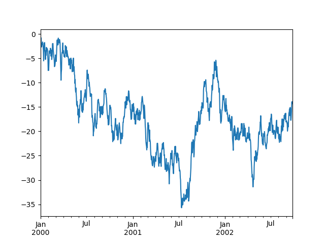
Note
When using Jupyter, the plot will appear using plot(). Otherwise use matplotlib.pyplot.show to show it or matplotlib.pyplot.savefig to write it to a file.
Jupyter를 사용하면 plot()을 사용하여 플롯이 나타난다. 그렇지 않으면 matplotlib.pyplot.show를 사용하여 표시하거나 matplotlib.pyplot.savefig를 사용하여 파일에 쓴다.
plot() plots all columns:
plot()은 모든 열을 플롯한다.
df = pd.DataFrame(
    np.random.randn(1000, 4), index=ts.index, columns=["A", "B", "C", "D"]
)

df = df.cumsum()

plt.figure();

df.plot();

plt.legend(loc='best');
Importing and exporting data
See the IO Tools section.
IO 도구 섹션을 참조한다.
CSV
Writing to a csv file: using DataFrame.to_csv()
csv 파일에 쓰기: DataFrame.to_csv() 사용
df = pd.DataFrame(np.random.randint(0, 5, (10, 5)))

df.to_csv("foo.csv")
Reading from a csv file: using read_csv()
csv 파일에서 읽기: read_csv() 사용
pd.read_csv("foo.csv")
Out[136]:
   Unnamed: 0  0  1  2  3  4
0           0  4  3  1  1  2
1           1  1  0  2  3  2
2           2  1  4  2  1  2
3           3  0  4  0  2  2
4           4  4  2  2  3  4
5           5  4  0  4  3  1
6           6  2  1  2  0  3
7           7  4  0  4  4  4
8           8  4  4  1  0  1
9           9  0  4  3  0  3
Parquet
Writing to a Parquet file:
Parquet 파일에 쓰기:
df.to_parquet("foo.parquet")Reading from a Parquet file Store using read_parquet():
read_parquet()를 사용하여 Parquet 파일 저장소에서 읽기:
pd.read_parquet("foo.parquet")
Out[138]:
   0  1  2  3  4
0  4  3  1  1  2
1  1  0  2  3  2
2  1  4  2  1  2
3  0  4  0  2  2
4  4  2  2  3  4
5  4  0  4  3  1
6  2  1  2  0  3
7  4  0  4  4  4
8  4  4  1  0  1
9  0  4  3  0  3
Excel
Reading and writing to Excel.
Writing to an excel file using DataFrame.to_excel():
Excel에서 읽고 쓰기.
DataFrame.to_excel()을 사용하여 Excel 파일에 쓰기:
df.to_excel("foo.xlsx", sheet_name="Sheet1")Reading from an excel file using read_excel():
read_excel()을 사용하여 Excel 파일에서 읽기:
pd.read_excel("foo.xlsx", "Sheet1", index_col=None, na_values=["NA"])
Out[140]:
   Unnamed: 0  0  1  2  3  4
0           0  4  3  1  1  2
1           1  1  0  2  3  2
2           2  1  4  2  1  2
3           3  0  4  0  2  2
4           4  4  2  2  3  4
5           5  4  0  4  3  1
6           6  2  1  2  0  3
7           7  4  0  4  4  4
8           8  4  4  1  0  1
9           9  0  4  3  0  3
Gotchas
If you are attempting to perform a boolean operation on a Series or DataFrame you might see an exception like:
Series 또는 DataFrame에서 부울 연산을 수행하려고 하면 다음과 같은 예외가 나타날 수 있다.
if pd.Series([False, True, False]):
     print("I was true")

---------------------------------------------------------------------------
ValueError                                Traceback (most recent call last)
 in ?()
----> 1 if pd.Series([False, True, False]):
      2      print("I was true")

~/work/pandas/pandas/pandas/core/generic.py in ?(self)
   1575     @final
   1576     def __nonzero__(self) -> NoReturn:
-> 1577         raise ValueError(
   1578             f"The truth value of a {type(self).__name__} is ambiguous. "
   1579             "Use a.empty, a.bool(), a.item(), a.any() or a.all()."
   1580         )

ValueError: The truth value of a Series is ambiguous. Use a.empty, a.bool(), a.item(), a.any() or a.all().
See Comparisons and Gotchas for an explanation and what to do.
728x90'코딩 > Python' 카테고리의 다른 글
Python/Pandas DataFrame에 대한 팁 (1) 2024.05.22 Python/통계에 따른 로또 번호 생성기 (2) 2024.05.09 Pyton/프로그램의 종료, exit() & quit() (0) 2024.04.17 Python/프로젝트 패키징 (1) 2024.03.15 Python/Reference/어휘분석 (1) 2024.03.15