-
Python/자연과학 데이터를 지도에 표시하는 basemap/User guide코딩/Python 2024. 7. 10. 14:33728x90
Basemap user guide의 번역본. 설치방법과 projection의 종류에 대해서는 제외.
Introduction
The matplotlib basemap toolkit is a library for plotting 2D data on maps in Python. It is similar in functionality to GrADS, GMT, the MATLAB Mapping Toolbox and the IDL Mapping Facilities. CDAT and PyNGL are other Python libraries with similar capabilities.
Basemap does not plot on its own, but provides the facilities to transform coordinates to one of 25 different map projections (using pyproj and therefore the PROJ C library). Then matplotlib is used to plot contours, images, vectors, lines or points in the transformed coordinates. Shoreline, river and political boundary datasets (extracted from GMT) are provided, together with methods for plotting them. The GEOS library is used internally to clip the coastline and political boundary features to the map projection region.
Basemap is geared towards the needs of Earth scientists, particularly oceanographers and meteorologists. Jeff Whitaker originally wrote Basemap to help in his research (climate and weather forecasting), since at the time CDAT was the only other tool in Python for plotting data on map projections. Over the years, the capabilities of basemap have evolved as scientists in other disciplines (such as biology, geology and geophysics) requested and contributed new features.
matplotlib 베이스맵 툴킷은 Python의 지도에 2D 데이터를 그리는 라이브러리이다. 기능면에서 GrADS, GMT, MATLAB Mapping Toolbox 및 IDL 매핑 기능과 유사하다. CDAT와 PyNGL은 비슷한 기능을 가진 다른 Python 라이브러리이다.
베이스맵은 자체적으로 플롯하지 않지만 좌표를 25개의 다른 지도 투영 중 하나로 변환하는 기능을 제공한다(pyproj 및 PROJ C 라이브러리 사용). 그런 다음 matplotlib를 사용하여 변환된 좌표에 윤곽선, 이미지, 벡터, 선 또는 점을 표시한다. 해안선, 강 및 정치적 경계 데이터 세트(GMT에서 추출)가 이를 표시하는 방법과 함께 제공된다. GEOS 라이브러리는 해안선과 정치적 경계 지형을 지도 투영 영역에 자르기 위해 내부적으로 사용된다.
베이스맵은 지구 과학자, 특히 해양학자와 기상학자의 요구에 맞춰 제작되었다. Jeff Whitaker는 원래 자신의 연구(기후 및 일기 예보)를 돕기 위해 Basemap을 작성했는데, 그 당시 CDAT는 지도 투영에 데이터를 표시하기 위한 Python의 유일한 도구였기 때문이다. 수년에 걸쳐 베이스맵의 기능은 다른 분야(예: 생물학, 지질학, 지구물리학)의 과학자들이 새로운 기능을 요청하고 기여함에 따라 발전해 왔다.
Setting up the map
Projection의 종류에 대해서는 제외한 번역본.
In order to represent the curved surface of the earth on a two-dimensional map, a map projection is needed. Since this cannot be done without distortion, there are many map projections, each with it’s own advantages and disadvantages. Basemap provides 24 different map projections. Some are global, some can only represent a portion of the globe. When a Basemap class instance is created, the desired map projection must be specified, along with information about the portion of the earth’s surface that the map projection will describe. There are two basic ways of doing this. One is to provide the latitude and longitude values of each of the four corners of the rectangular map projection region. The other is to provide the lat/lon value of the center of the map projection region along with the width and height of the region in map projection coordinates.
The class variable supported_projections is a dictionary containing information about all the projections supported by Basemap. The keys are the short names (used with the projection keyword to define a projection when creating a Basemap class instance), and the values are longer, more descriptive names. The class variable projection_params is a dictionary that provides a list of parameters that can be used to define the properties of each projection. Following are examples that illustrate how to set up each of the supported projections. Note that many map projection possess one of two desirable properties - they can be equal-area (the area of features is preserved) or conformal (the shape of features is preserved). Since no map projection can have both at the same time, many compromise between the two.
지구의 곡면을 2차원 지도에 표현하기 위해서는 지도 투영법이 필요하다. 왜곡 없이는 이 작업을 수행할 수 없기 때문에 지도 투영법이 많이 있으며 각각 고유한 장점과 단점이 있다. 베이스맵은 24가지 지도 투영을 제공한다. 일부는 글로벌하고 일부는 지구의 일부만 나타낼 수 있다. Basemap 클래스 인스턴스가 생성되면 지도 투영이 설명할 지구 표면 부분에 대한 정보와 함께 원하는 지도 투영을 지정해야 한다. 이를 수행하는 두 가지 기본 방법이 있다. 하나는 직사각형 지도 투영 영역의 네 모서리 각각에 대한 위도 및 경도 값을 제공하는 것이다. 다른 하나는 지도 투영 좌표에 해당 지역의 너비와 높이와 함께 지도 투영 지역 중심의 위도/경도 값을 제공하는 것이다.
클래스 변수 supported_projections는 Basemap에서 지원하는 모든 투영에 대한 정보가 포함된 dictionary이다. key는 짧은 이름(Basemap 클래스 인스턴스를 생성할 때 투영을 정의하기 위해 투영 키워드와 함께 사용됨)이고 value는 더 길고 설명이 포함된 이름이다. 클래스 변수 projection_params는 각 투영의 속성을 정의하는 데 사용할 수 있는 매개 변수 목록을 제공하는 dictionary이다. 다음은 지원되는 각 투영을 설정하는 방법을 보여주는 예이다. 많은 지도 투영법은 두 가지 바람직한 속성 중 하나를 가지고 있다. 즉, 동일 면적(지형의 면적이 보존됨) 또는 등각(지형의 모양이 보존됨)일 수 있다. 어떤 지도 투영도 두 가지를 동시에 가질 수 없기 때문에 많은 사람들이 둘 사이에서 절충한다.
Drawing a Map Background
Basemap includes the GSHHG coastline dataset, as well as datasets for rivers, state and country boundaries from GMT. These datasets can be used to draw coastlines, rivers and political boundaries on maps at several different resolutions. The relevant Basemap methods are:
- drawcoastlines(): draw coastlines.
- fillcontinents(): color the interior of continents (by filling the coastline polygons). Unfortunately, the fillcontinents method doesn’t always do the right thing. Matplotlib always tries to fill the inside of a polygon. Under certain situations, what is the inside of a coastline polygon can be ambiguous, and the outside may be filled instead of the inside. In these situations, the recommended workaround is to use the drawlsmask() method to overlay an image with different colors specified for land and water regions (see below).
- drawcountries(): draw country boundaries.
- drawstates(): draw state boundaries in North America.
- drawrivers(): draw rivers.
베이스맵에는 GSHHG 해안선 데이터세트와 GMT의 강, 주, 국가 경계에 대한 데이터세트가 포함되어 있다. 이러한 데이터 세트는 다양한 해상도로 지도에 해안선, 강, 정치적 경계를 그리는 데 사용할 수 있다. 관련 베이스맵 메소드는 다음과 같다:
- drawcoastlines(): 해안선을 그린다.
- fillcontinents(): 대륙 내부를 색칠한다(해안선 다각형을 채워서). 불행하게도 fillcontinents 메서드가 항상 올바른 작업을 수행하는 것은 아니다. Matplotlib는 항상 다각형 내부를 채우려고 한다. 특정 상황에서는 해안선 다각형의 내부가 무엇인지 모호할 수 있으며 내부가 아닌 외부가 채워질 수 있다. 이러한 상황에서 권장되는 해결 방법은 drawlsmask() 메서드를 사용하여 육지와 바다 지역에 대해 지정된 다양한 색상으로 이미지를 오버레이하는 것이다(아래 참조).
- drawcountries(): 국가 경계를 그린다.
- drawstates(): 북미의 주 경계를 그린다.
- drawrivers(): 강을 그린다.
Instead of drawing coastlines and political boundaries, an image can be used as a map background. Basemap provides several options for this:
- drawlsmask(): draw a high-resolution land-sea mask as an image, with land and ocean colors specified. The land-sea mask is derived from the GSHHS coastline data, and there are several coastline options and pixel sizes to choose from.
- bluemarble(): draw a NASA Blue Marble image as a map background.
- shadedrelief(): draw a shaded relief image as a map background.
- etopo(): draw an etopo relief image as map background.
- warpimage(): use an abitrary image as a map background. The image must be global, covering the world in lat/lon coordinates from the international dateline eastward and the South Pole northward.
해안선이나 정치적 경계를 그리는 대신 이미지를 지도 배경으로 사용할 수 있다. 베이스맵은 이에 대한 몇 가지 옵션을 제공한다.
- drawlsmask(): 지정된 육지 및 바다 색상을 사용하여 고해상도 육지-해양 마스크를 이미지로 그린다. 육지-해양 마스크는 GSHHS 해안선 데이터에서 파생되며 선택할 수 있는 여러 해안선 옵션과 픽셀 크기가 있다.
- bluemarble(): NASA Blue Marble 이미지를 지도 배경으로 그린다.
- Shadrelief(): 음영 기복 이미지를 지도 배경으로 그린다.
- etopo(): 지도 배경으로 etopo 부조 이미지를 그린다.
- warpimage(): 임의의 이미지를 지도 배경으로 사용한다. 이미지는 국제 날짜 변경선에서 동쪽으로, 남극에서 북쪽으로 위도/경도 좌표로 세계를 포괄하는 전역적이어야 하다.
Here are examples of the various ways to draw a map background.
다음은 지도 배경을 그리는 다양한 방법의 예이다.
1. Draw coastlines, filling ocean and land areas.
1. 해안선을 그려 바다와 육지를 채운다.
from mpl_toolkits.basemap import Basemap
import matplotlib.pyplot as plt
# setup Lambert Conformal basemap.
m = Basemap(width=12000000,height=9000000,projection='lcc',
            resolution='c',lat_1=45.,lat_2=55,lat_0=50,lon_0=-107.)
# draw coastlines.
m.drawcoastlines()
# draw a boundary around the map, fill the background.
# this background will end up being the ocean color, since
# the continents will be drawn on top.
m.drawmapboundary(fill_color='aqua')
# fill continents, set lake color same as ocean color.
m.fillcontinents(color='coral',lake_color='aqua')
plt.show()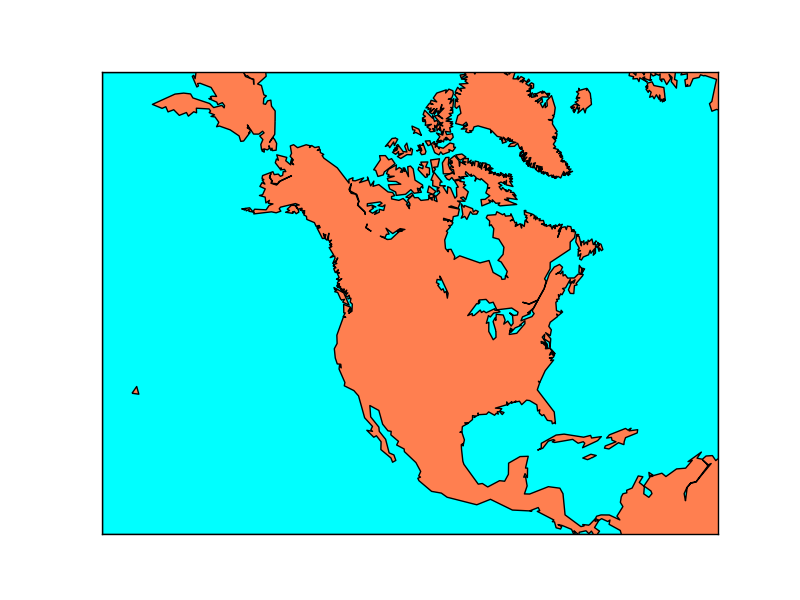
2. Draw a land-sea mask as an image.
2. 육지-바다 마스크를 이미지로 그린다.
from mpl_toolkits.basemap import Basemap
import matplotlib.pyplot as plt
# setup Lambert Conformal basemap.
# set resolution=None to skip processing of boundary datasets.
m = Basemap(width=12000000,height=9000000,projection='lcc',
            resolution=None,lat_1=45.,lat_2=55,lat_0=50,lon_0=-107.)
# draw a land-sea mask for a map background.
# lakes=True means plot inland lakes with ocean color.
m.drawlsmask(land_color='coral',ocean_color='aqua',lakes=True)
plt.show()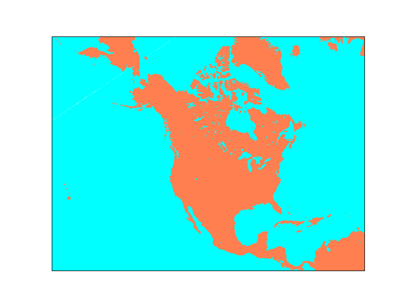
3. Draw the NASA ‘Blue Marble’ image.
3. NASA의 'Blue Marble' 이미지를 그린다.
from mpl_toolkits.basemap import Basemap
import matplotlib.pyplot as plt
# setup Lambert Conformal basemap.
# set resolution=None to skip processing of boundary datasets.
m = Basemap(width=12000000,height=9000000,projection='lcc',
            resolution=None,lat_1=45.,lat_2=55,lat_0=50,lon_0=-107.)
m.bluemarble()
plt.show()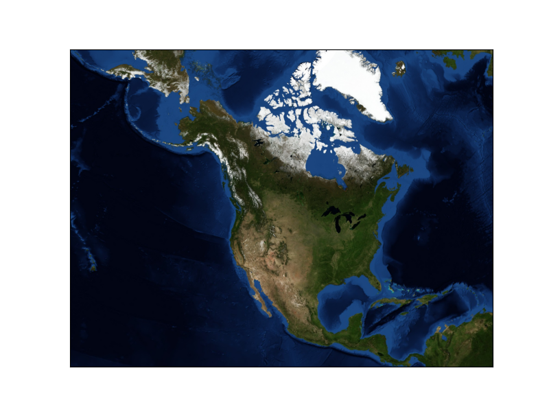
4. Draw a shaded relief image.
4. shaded relief 이미지를 그린다.
from mpl_toolkits.basemap import Basemap
import matplotlib.pyplot as plt
# setup Lambert Conformal basemap.
# set resolution=None to skip processing of boundary datasets.
m = Basemap(width=12000000,height=9000000,projection='lcc',
            resolution=None,lat_1=45.,lat_2=55,lat_0=50,lon_0=-107.)
m.shadedrelief()
plt.show()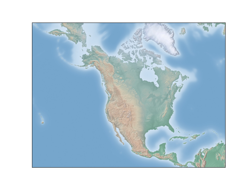
5. Draw an etopo relief image.
5. etopo relief 이미지를 그린다.
from mpl_toolkits.basemap import Basemap
import matplotlib.pyplot as plt
# setup Lambert Conformal basemap.
# set resolution=None to skip processing of boundary datasets.
m = Basemap(width=12000000,height=9000000,projection='lcc',
            resolution=None,lat_1=45.,lat_2=55,lat_0=50,lon_0=-107.)
m.etopo()
plt.show()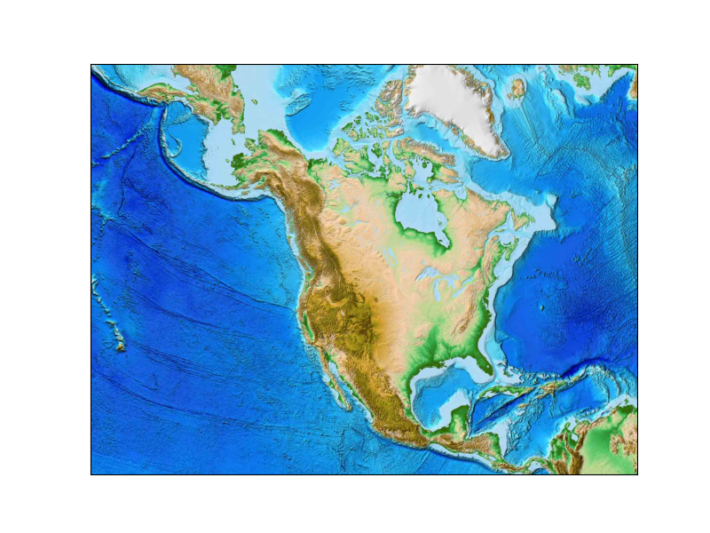
Drawing and Labelling Parallels and Meridians
Most maps include a graticule grid, a reference network of labelled latitude and longitude lines. Basemap does this with the drawparallels() and drawmeridians() instance methods. The longitude and latitude lines can be labelled where they intersect the map projection boundary. There are a few exceptions: meridians and parallels cannot be labelled on maps with proj set to ortho (orthographic), geos (geostationary), vandg (van der Grinten) or nsper (near-sided perspective), and meridians cannot be labelled on maps with proj set to ortho (orthographic), geos (geostationary), vandg (van der Grinten), nsper (near-sided perspective), moll (Mollweide), hammer (Hammer), or sinu (sinusoidal). This is because the lines can be very close together where they intersect the boundary on these maps, so that they really need to be labelled manually on the interior of the plot. Here’s an example that shows how to draw parallels and meridians and label them on different sides of the plot.
대부분의 지도에는 레이블이 지정된 위도 및 경도 선의 참조 네트워크인 계수선 그리드가 포함되어 있다. Basemap은 drawparallels() 및 drawmeridians() 인스턴스 메서드를 사용하여 이 작업을 수행한다. 경도 및 위도 선은 지도 투영 경계와 교차하는 위치에 라벨을 붙일 수 있다. 몇 가지 예외가 있다. 프로젝트가 직교(정교), geos(정지궤도), vandg(van der Grinten) 또는 nsper(근접 원근법)로 설정된 지도에서는 자오선과 평행선에 라벨을 붙일 수 없으며 자오선은 지도에 라벨을 붙일 수 없다. 프로젝트를 직교(직교), geos(정지궤도), vandg(van der Grinten), nsper(근접 원근법), moll(Mollweide), hammer(해머) 또는 sinu(정현파)로 설정한다. 이는 지도의 경계와 교차하는 선이 서로 매우 가까울 수 있기 때문에 플롯 내부에서 수동으로 라벨을 지정해야 하기 때문이다. 다음은 평행선과 자오선을 그리고 플롯의 다른 측면에 레이블을 지정하는 방법을 보여주는 예이다.
from mpl_toolkits.basemap import Basemap
import matplotlib.pyplot as plt
import numpy as np
# setup Lambert Conformal basemap.
m = Basemap(width=12000000,height=9000000,projection='lcc',
            resolution='c',lat_1=45.,lat_2=55,lat_0=50,lon_0=-107.)
# draw coastlines.
m.drawcoastlines()
# draw a boundary around the map, fill the background.
# this background will end up being the ocean color, since
# the continents will be drawn on top.
m.drawmapboundary(fill_color='aqua')
# fill continents, set lake color same as ocean color.
m.fillcontinents(color='coral',lake_color='aqua')
# draw parallels and meridians.
# label parallels on right and top
# meridians on bottom and left
parallels = np.arange(0.,81,10.)
# labels = [left,right,top,bottom]
m.drawparallels(parallels,labels=[False,True,True,False])
meridians = np.arange(10.,351.,20.)
m.drawmeridians(meridians,labels=[True,False,False,True])
plt.show()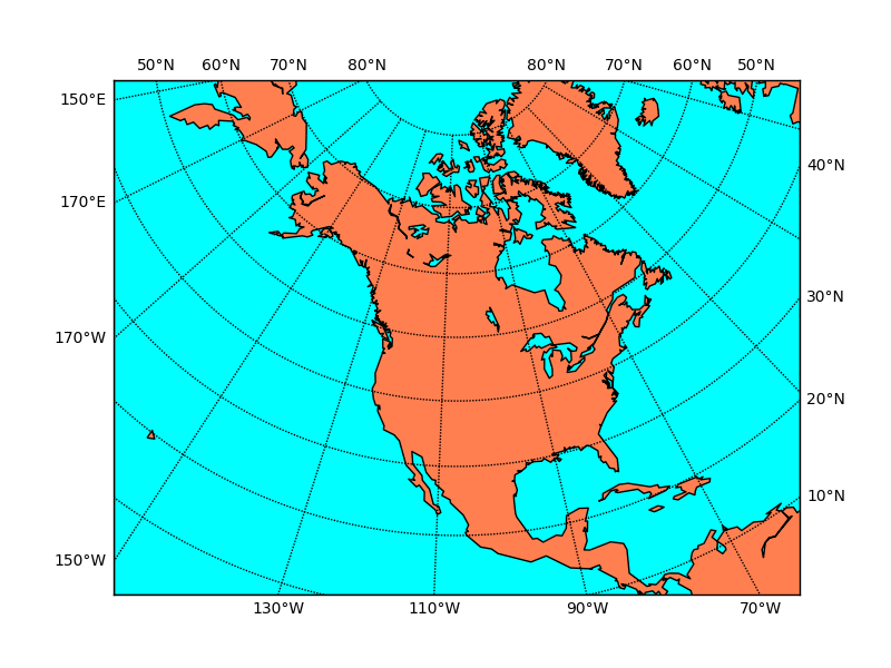
Converting to and from map projection coordinates
In order to plot data on a map, the coordinates of the data must be given in map projection coordinates. Calling a Basemap class instance with the arguments lon, lat will convert lon/lat (in degrees) to x/y map projection coordinates (in meters). The inverse transformation is done if the optional keyword inverse is set to True. Here’s an example that uses this feature to plot a marker and some text to denote the location of Boulder, CO, given the lat/lon position.
지도에 데이터를 표시하려면 데이터의 좌표가 지도 투영 좌표로 제공되어야 한다. lon 인수를 사용하여 Basemap 클래스 인스턴스를 호출하면 lat는 lon/lat(도 단위)를 x/y 지도 투영 좌표(미터 단위)로 변환한다. 선택적 키워드 inverse가 True로 설정된 경우 역변환이 수행된다. 다음은 이 기능을 사용하여 위도/경도 위치를 기준으로 콜로라도 주 Boulder의 위치를 나타내는 마커와 일부 텍스트를 표시하는 예이다.
from mpl_toolkits.basemap import Basemap
import matplotlib.pyplot as plt
import numpy as np
# setup Lambert Conformal basemap.
m = Basemap(width=12000000,height=9000000,projection='lcc',
            resolution='c',lat_1=45.,lat_2=55,lat_0=50,lon_0=-107.)
# draw a boundary around the map, fill the background.
# this background will end up being the ocean color, since
# the continents will be drawn on top.
m.drawmapboundary(fill_color='aqua')
# fill continents, set lake color same as ocean color.
m.fillcontinents(color='coral',lake_color='aqua')
# draw parallels and meridians.
# label parallels on right and top
# meridians on bottom and left
parallels = np.arange(0.,81,10.)
# labels = [left,right,top,bottom]
m.drawparallels(parallels,labels=[False,True,True,False])
meridians = np.arange(10.,351.,20.)
m.drawmeridians(meridians,labels=[True,False,False,True])
# plot blue dot on Boulder, colorado and label it as such.
lon, lat = -104.237, 40.125 # Location of Boulder
# convert to map projection coords.
# Note that lon,lat can be scalars, lists or numpy arrays.
xpt,ypt = m(lon,lat)
# convert back to lat/lon
lonpt, latpt = m(xpt,ypt,inverse=True)
m.plot(xpt,ypt,'bo')  # plot a blue dot there
# put some text next to the dot, offset a little bit
# (the offset is in map projection coordinates)
plt.text(xpt+100000,ypt+100000,'Boulder (%5.1fW,%3.1fN)' % (lonpt,latpt))
plt.show()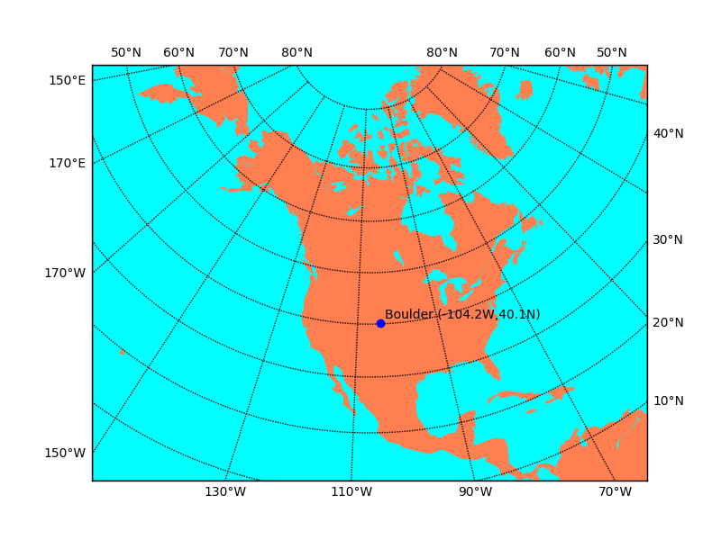
Plotting data on a map (Example Gallery)
Following are a series of examples that illustrate how to use Basemap instance methods to plot your data on a map. More examples are included in the examples directory of the basemap source distribution. There are a number of Basemap instance methods for plotting data:
- contour(): draw contour lines.
- contourf(): draw filled contours.
- imshow(): draw an image.
- pcolor(): draw a pseudocolor plot.
- pcolormesh(): draw a pseudocolor plot (faster version for regular meshes).
- plot(): draw lines and/or markers.
- scatter(): draw points with markers.
- quiver(): draw vectors.
- barbs(): draw wind barbs.
- drawgreatcircle(): draw a great circle.
다음은 Basemap 인스턴스 메소드를 사용하여 지도에 데이터를 그리는 방법을 보여주는 일련의 예이다. 베이스맵 소스 배포의 예제 디렉터리에 더 많은 예제가 포함되어 있다. 데이터를 그리는 데는 여러 가지 Basemap 인스턴스 메소드가 있다.
- contour(): 등고선을 그린다.
- contourf(): 채워진 윤곽선을 그린다.
- imshow(): 이미지를 그린다.
- pcolor(): 의사색상 플롯을 그린다.
- pcolormesh(): 유사 색상 플롯을 그린다(일반 메시의 경우 더 빠른 버전).
- plot(): 선 및/또는 마커를 그린다.
- scatter(): 마커로 점을 그린다.
- quiver(): 벡터를 그린다.
- barbs(): 바람 미늘을 그린다.
- drawgreatcircle(): 큰 원을 그린다.
Many of these instances methods simply forward to the corresponding matplotlib Axes instance method, with some extra pre/post processing and argument checking. You can also plot on the map directly with the matplotlib pyplot interface, or the OO api, using the Axes instance associated with the Basemap.
For more specifics of how to use the Basemap instance methods, see Basemap API.
Here are the examples (many of which utilize the netcdf4-python module to retrieve datasets over http):
이러한 인스턴스 메서드 중 다수는 추가 사전/사후 처리 및 인수 확인을 통해 해당 matplotlib Axes 인스턴스 메서드로 전달된다. 또한 기본 지도와 연결된 Axes 인스턴스를 사용하여 matplotlib pyplot 인터페이스 또는 OO API를 사용하여 지도에 직접 플롯할 수도 있다.
Basemap 인스턴스 메소드를 사용하는 방법에 대한 자세한 내용은 Basemap API를 참조하라.
다음은 예제이다(대다수는 http를 통해 데이터세트를 검색하기 위해 netcdf4-python 모듈을 사용한다):
- Plot contour lines on a basemap
- 베이스맵에 등고선 플롯
from mpl_toolkits.basemap import Basemap
import matplotlib.pyplot as plt
import numpy as np
# set up orthographic map projection with
# perspective of satellite looking down at 45N, 100W.
# use low resolution coastlines.
map = Basemap(projection='ortho',lat_0=45,lon_0=-100,resolution='l')
# draw coastlines, country boundaries, fill continents.
map.drawcoastlines(linewidth=0.25)
map.drawcountries(linewidth=0.25)
map.fillcontinents(color='coral',lake_color='aqua')
# draw the edge of the map projection region (the projection limb)
map.drawmapboundary(fill_color='aqua')
# draw lat/lon grid lines every 30 degrees.
map.drawmeridians(np.arange(0,360,30))
map.drawparallels(np.arange(-90,90,30))
# make up some data on a regular lat/lon grid.
nlats = 73; nlons = 145; delta = 2.*np.pi/(nlons-1)
lats = (0.5*np.pi-delta*np.indices((nlats,nlons))[0,:,:])
lons = (delta*np.indices((nlats,nlons))[1,:,:])
wave = 0.75*(np.sin(2.*lats)**8*np.cos(4.*lons))
mean = 0.5*np.cos(2.*lats)*((np.sin(2.*lats))**2 + 2.)
# compute native map projection coordinates of lat/lon grid.
x, y = map(lons*180./np.pi, lats*180./np.pi)
# contour data over the map.
cs = map.contour(x,y,wave+mean,15,linewidths=1.5)
plt.title('contour lines over filled continent background')
plt.show()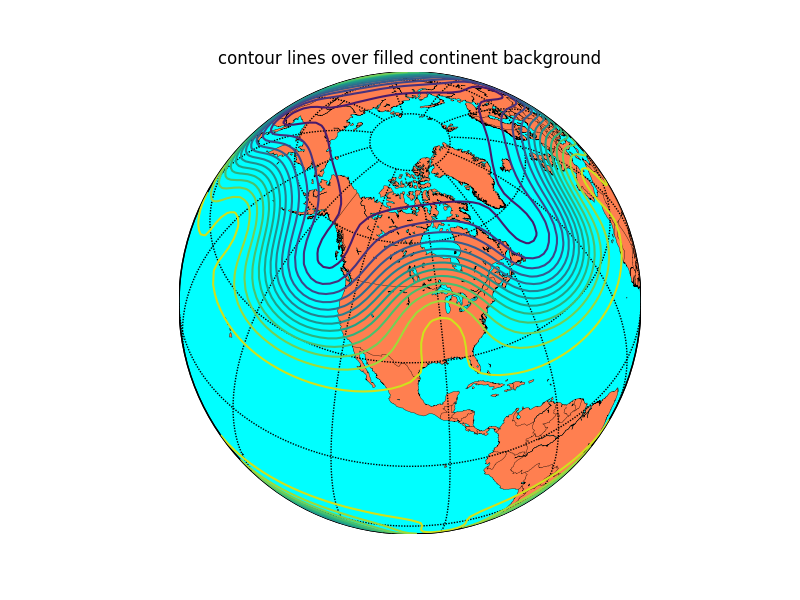
- Plot precip with filled contours
- 채워진 등고선으로 강수량 플롯
from mpl_toolkits.basemap import Basemap, cm
# requires netcdf4-python (netcdf4-python.googlecode.com)
from netCDF4 import Dataset as NetCDFFile
import os
import numpy as np
import matplotlib.pyplot as plt

# plot rainfall from NWS using special precipitation
# colormap used by the NWS, and included in basemap.

ncpath = os.path.join(*6 * [".."] + ["examples", "nws_precip_conus_20061222.nc"])
nc = NetCDFFile(ncpath)
# data from http://water.weather.gov/precip/
prcpvar = nc.variables['amountofprecip']
data = 0.01*prcpvar[:]
latcorners = nc.variables['lat'][:]
loncorners = -nc.variables['lon'][:]
lon_0 = -nc.variables['true_lon'].getValue()
lat_0 = nc.variables['true_lat'].getValue()
# create figure and axes instances
fig = plt.figure(figsize=(8,8))
ax = fig.add_axes([0.1,0.1,0.8,0.8])
# create polar stereographic Basemap instance.
m = Basemap(projection='stere',lon_0=lon_0,lat_0=90.,lat_ts=lat_0,\
            llcrnrlat=latcorners[0],urcrnrlat=latcorners[2],\
            llcrnrlon=loncorners[0],urcrnrlon=loncorners[2],\
            rsphere=6371200.,resolution='l',area_thresh=10000)
# draw coastlines, state and country boundaries, edge of map.
m.drawcoastlines()
m.drawstates()
m.drawcountries()
# draw parallels.
parallels = np.arange(0.,90,10.)
m.drawparallels(parallels,labels=[1,0,0,0],fontsize=10)
# draw meridians
meridians = np.arange(180.,360.,10.)
m.drawmeridians(meridians,labels=[0,0,0,1],fontsize=10)
ny = data.shape[0]; nx = data.shape[1]
lons, lats = m.makegrid(nx, ny) # get lat/lons of ny by nx evenly space grid.
x, y = m(lons, lats) # compute map proj coordinates.
# draw filled contours.
clevs = [0,1,2.5,5,7.5,10,15,20,30,40,50,70,100,150,200,250,300,400,500,600,750]
cs = m.contourf(x,y,data,clevs,cmap=cm.s3pcpn)
# add colorbar.
cbar = m.colorbar(cs,location='bottom',pad="5%")
cbar.set_label('mm')
# add title
plt.title(prcpvar.long_name+' for period ending '+prcpvar.dateofdata)
plt.show()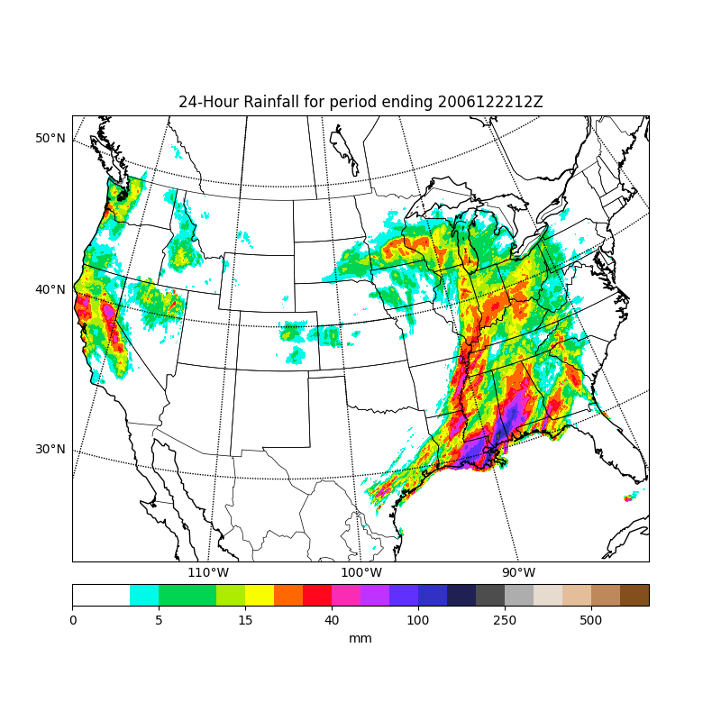
- Plot sea-level pressure weather map with labelled highs and lows
- 최고 및 최저 라벨이 표시된 해수면 기압 기상 지도 그리기
"""
plot H's and L's on a sea-level pressure map
(uses scipy.ndimage.filters and netcdf4-python)
"""
import numpy as np
import matplotlib.pyplot as plt
from datetime import datetime
from mpl_toolkits.basemap import Basemap, addcyclic
from scipy.ndimage.filters import minimum_filter, maximum_filter
from netCDF4 import Dataset

def extrema(mat,mode='wrap',window=10):
    """find the indices of local extrema (min and max)
    in the input array."""
    mn = minimum_filter(mat, size=window, mode=mode)
    mx = maximum_filter(mat, size=window, mode=mode)
    # (mat == mx) true if pixel is equal to the local max
    # (mat == mn) true if pixel is equal to the local in
    # Return the indices of the maxima, minima
    return np.nonzero(mat == mn), np.nonzero(mat == mx)

# plot 00 UTC today.
date = datetime.now().strftime('%Y%m%d')+'00'

# open OpenDAP dataset.
data=Dataset("https://nomads.ncep.noaa.gov/dods/gfs_0p50/gfs%s/gfs_0p50_%sz"%\
        (date[0:8],date[8:10]))

# read lats,lons.
lats = data.variables['lat'][:]
lons1 = data.variables['lon'][:]
nlats = len(lats)
nlons = len(lons1)
# read prmsl, convert to hPa (mb).
prmsl = 0.01*data.variables['prmslmsl'][0]
# the window parameter controls the number of highs and lows detected.
# (higher value, fewer highs and lows)
local_min, local_max = extrema(prmsl, mode='wrap', window=50)
# create Basemap instance.
m =\
Basemap(llcrnrlon=0,llcrnrlat=-80,urcrnrlon=360,urcrnrlat=80,projection='mill')
# add wrap-around point in longitude.
prmsl, lons = addcyclic(prmsl, lons1)
# contour levels
clevs = np.arange(900,1100.,5.)
# find x,y of map projection grid.
lons, lats = np.meshgrid(lons, lats)
x, y = m(lons, lats)
# create figure.
fig=plt.figure(figsize=(8,4.5))
ax = fig.add_axes([0.05,0.05,0.9,0.85])
cs = m.contour(x,y,prmsl,clevs,colors='k',linewidths=1.)
m.drawcoastlines(linewidth=1.25)
m.fillcontinents(color='0.8')
m.drawparallels(np.arange(-80,81,20),labels=[1,1,0,0])
m.drawmeridians(np.arange(0,360,60),labels=[0,0,0,1])
xlows = x[local_min]; xhighs = x[local_max]
ylows = y[local_min]; yhighs = y[local_max]
lowvals = prmsl[local_min]; highvals = prmsl[local_max]
# plot lows as blue L's, with min pressure value underneath.
xyplotted = []
# don't plot if there is already a L or H within dmin meters.
yoffset = 0.022*(m.ymax-m.ymin)
dmin = yoffset
for x,y,p in zip(xlows, ylows, lowvals):
    if x < m.xmax and x > m.xmin and y < m.ymax and y > m.ymin:
        dist = [np.sqrt((x-x0)2+(y-y0)2) for x0,y0 in xyplotted]
        if not dist or min(dist) > dmin:
            plt.text(x,y,'L',fontsize=14,fontweight='bold',
                    ha='center',va='center',color='b')
            plt.text(x,y-yoffset,repr(int(p)),fontsize=9,
                    ha='center',va='top',color='b',
                    bbox = dict(boxstyle="square",ec='None',fc=(1,1,1,0.5)))
            xyplotted.append((x,y))
# plot highs as red H's, with max pressure value underneath.
xyplotted = []
for x,y,p in zip(xhighs, yhighs, highvals):
    if x < m.xmax and x > m.xmin and y < m.ymax and y > m.ymin:
        dist = [np.sqrt((x-x0)2+(y-y0)2) for x0,y0 in xyplotted]
        if not dist or min(dist) > dmin:
            plt.text(x,y,'H',fontsize=14,fontweight='bold',
                    ha='center',va='center',color='r')
            plt.text(x,y-yoffset,repr(int(p)),fontsize=9,
                    ha='center',va='top',color='r',
                    bbox = dict(boxstyle="square",ec='None',fc=(1,1,1,0.5)))
            xyplotted.append((x,y))
plt.title('Mean Sea-Level Pressure (with Highs and Lows) %s' % date)
plt.show()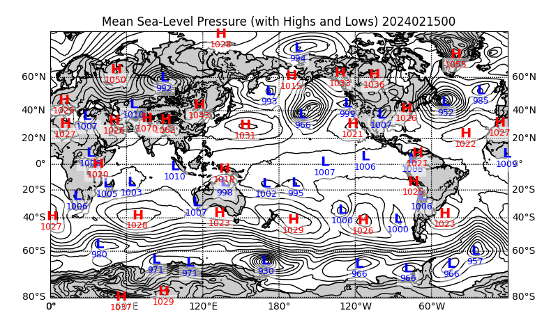
- Plot hurricane tracks from a shapefile
- shapefile에서 허리케인 트랙을 플롯.
"""
draw Atlantic Hurricane Tracks for storms that reached Cat 4 or 5.
part of the track for which storm is cat 4 or 5 is shown red.
ESRI shapefile data from http://nationalatlas.gov/mld/huralll.html
"""
import os
import numpy as np
import matplotlib.pyplot as plt
from mpl_toolkits.basemap import Basemap
# Lambert Conformal Conic map.
m = Basemap(llcrnrlon=-100.,llcrnrlat=0.,urcrnrlon=-20.,urcrnrlat=57.,
            projection='lcc',lat_1=20.,lat_2=40.,lon_0=-60.,
            resolution ='l',area_thresh=1000.)
# read shapefile.
shp_path = os.path.join(*6 * [".."] + ["examples", "huralll020"])
shp_info = m.readshapefile(shp_path,'hurrtracks',drawbounds=False)
# find names of storms that reached Cat 4.
names = []
for shapedict in m.hurrtracks_info:
    cat = shapedict['CATEGORY']
    name = shapedict['NAME']
    if cat in ['H4','H5'] and name not in names:
        # only use named storms.
        if name != 'NOT NAMED':  names.append(name)
# plot tracks of those storms.
for shapedict,shape in zip(m.hurrtracks_info,m.hurrtracks):
    name = shapedict['NAME']
    cat = shapedict['CATEGORY']
    if name in names:
        xx,yy = zip(*shape)
        # show part of track where storm > Cat 4 as thick red.
        if cat in ['H4','H5']:
            m.plot(xx,yy,linewidth=1.5,color='r')
        elif cat in ['H1','H2','H3']:
            m.plot(xx,yy,color='k')
# draw coastlines, meridians and parallels.
m.drawcoastlines()
m.drawcountries()
m.drawmapboundary(fill_color='#99ffff')
m.fillcontinents(color='#cc9966',lake_color='#99ffff')
m.drawparallels(np.arange(10,70,20),labels=[1,1,0,0])
m.drawmeridians(np.arange(-100,0,20),labels=[0,0,0,1])
plt.title('Atlantic Hurricane Tracks (Storms Reaching Category 4, 1851-2004)')
plt.show()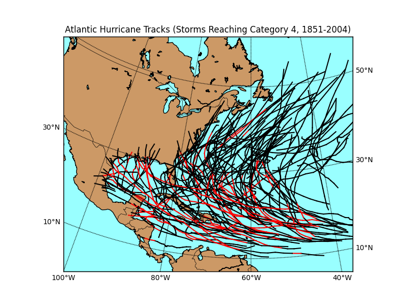
- Plot etopo5 topography/bathymetry data as an image (with and without shading from a specified light source).
- etopo5 지형/수심측량 데이터를 이미지로 플롯(지정된 광원의 음영 포함 및 제외).
from mpl_toolkits.basemap import Basemap, shiftgrid, cm
import numpy as np
import matplotlib.pyplot as plt
from netCDF4 import Dataset

# read in etopo5 topography/bathymetry.
url = 'http://ferret.pmel.noaa.gov/thredds/dodsC/data/PMEL/etopo5.nc'
etopodata = Dataset(url)

topoin = etopodata.variables['ROSE'][:]
lons = etopodata.variables['ETOPO05_X'][:]
lats = etopodata.variables['ETOPO05_Y'][:]
# shift data so lons go from -180 to 180 instead of 20 to 380.
topoin,lons = shiftgrid(180.,topoin,lons,start=False)

# plot topography/bathymetry as an image.

# create the figure and axes instances.
fig = plt.figure()
ax = fig.add_axes([0.1,0.1,0.8,0.8])
# setup of basemap ('lcc' = lambert conformal conic).
# use major and minor sphere radii from WGS84 ellipsoid.
m = Basemap(llcrnrlon=-145.5,llcrnrlat=1.,urcrnrlon=-2.566,urcrnrlat=46.352,\
            rsphere=(6378137.00,6356752.3142),\
            resolution='l',area_thresh=1000.,projection='lcc',\
            lat_1=50.,lon_0=-107.,ax=ax)
# transform to nx x ny regularly spaced 5km native projection grid
nx = int((m.xmax-m.xmin)/5000.)+1; ny = int((m.ymax-m.ymin)/5000.)+1
topodat = m.transform_scalar(topoin,lons,lats,nx,ny)
# plot image over map with imshow.
im = m.imshow(topodat,cm.GMT_haxby)
# draw coastlines and political boundaries.
m.drawcoastlines()
m.drawcountries()
m.drawstates()
# draw parallels and meridians.
# label on left and bottom of map.
parallels = np.arange(0.,80,20.)
m.drawparallels(parallels,labels=[1,0,0,1])
meridians = np.arange(10.,360.,30.)
m.drawmeridians(meridians,labels=[1,0,0,1])
# add colorbar
cb = m.colorbar(im,"right", size="5%", pad='2%')
ax.set_title('ETOPO5 Topography - Lambert Conformal Conic')
plt.show()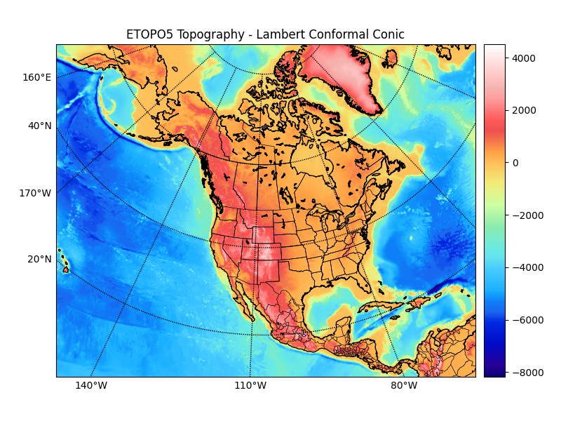
# make a shaded relief plot.

# create new figure, axes instance.
fig = plt.figure()
ax = fig.add_axes([0.1,0.1,0.8,0.8])
# attach new axes image to existing Basemap instance.
m.ax = ax
# create light source object.
from matplotlib.colors import LightSource
ls = LightSource(azdeg = 90, altdeg = 20)
# convert data to rgb array including shading from light source.
# (must specify color map)
rgb = ls.shade(topodat, cm.GMT_haxby)
im = m.imshow(rgb)
# draw coastlines and political boundaries.
m.drawcoastlines()
m.drawcountries()
m.drawstates()
ax.set_title('Shaded ETOPO5 Topography - Lambert Conformal Conic')
plt.show()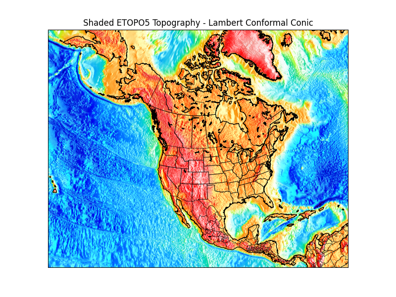
- Plot markers at locations of ARGO floats.
- ARGO floats 위치에 마커를 표시한다.
from netCDF4 import Dataset, num2date
import time, calendar, datetime, numpy
from mpl_toolkits.basemap import Basemap
import matplotlib.pyplot as plt
import os
try:
    from urllib.request import urlretrieve
except ImportError:
    from urllib import urlretrieve
# data downloaded from the form at
# http://coastwatch.pfeg.noaa.gov/erddap/tabledap/apdrcArgoAll.html
filename, headers = urlretrieve("https://erddap.ifremer.fr/erddap/tabledap/ArgoFloats-index.nc?date%2Clatitude%2Clongitude&date%3E=2010-01-01&date%3C=2010-01-08&latitude%3E=-90&latitude%3C=90&longitude%3E=-180&longitude%3C=180&distinct()")
dset = Dataset(filename)
lats = dset.variables['latitude'][:]
lons = dset.variables['longitude'][:]
time = dset.variables['date']  # seconds since epoch
times = time[:]
t1 = times.min(); t2 = times.max()
date1 = num2date(t1, units=time.units)
date2 = num2date(t2, units=time.units)
dset.close()
os.remove(filename)
# draw map with markers for float locations
m = Basemap(projection='hammer',lon_0=180)
x, y = m(lons,lats)
m.drawmapboundary(fill_color='#99ffff')
m.fillcontinents(color='#cc9966',lake_color='#99ffff')
m.scatter(x,y,3,marker='o',color='k')
plt.title('Locations of %s ARGO floats active between %s and %s' %\
        (len(lats),date1,date2),fontsize=12)
plt.show()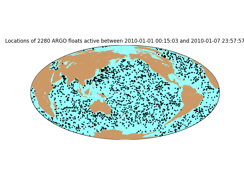
- Pseudo-color plot of SST and sea ice analysis.
- SST 및 해빙 분석의 Pseudo-color 플롯.
from mpl_toolkits.basemap import Basemap
from netCDF4 import Dataset, date2index
import numpy as np
import matplotlib.pyplot as plt
from datetime import datetime
try:
    from urllib.request import urlretrieve
except ImportError:
    from urllib import urlretrieve
date = datetime(2007,12,15,0) # date to plot.
# open dataset.
sstpath, sstheader = urlretrieve("https://downloads.psl.noaa.gov/Datasets/noaa.oisst.v2.highres/sst.day.mean.{0}.nc".format(date.year))
dataset = Dataset(sstpath)
timevar = dataset.variables['time']
timeindex = date2index(date,timevar) # find time index for desired date.
# read sst.  Will automatically create a masked array using
# missing_value variable attribute. 'squeeze out' singleton dimensions.
sst = dataset.variables['sst'][timeindex,:].squeeze()
# read ice.
dataset.close()
icepath, iceheader = urlretrieve("https://downloads.psl.noaa.gov/Datasets/noaa.oisst.v2.highres/icec.day.mean.{0}.nc".format(date.year))
dataset = Dataset(icepath)
ice = dataset.variables['icec'][timeindex,:].squeeze()
# read lats and lons (representing centers of grid boxes).
lats = dataset.variables['lat'][:]
lons = dataset.variables['lon'][:]
dataset.close()
latstep, lonstep = np.diff(lats[:2]), np.diff(lons[:2])
lats = np.append(lats - 0.5 * latstep, lats[-1] + 0.5 * latstep)
lons = np.append(lons - 0.5 * lonstep, lons[-1] + 0.5 * lonstep)
lons, lats = np.meshgrid(lons,lats)
# create figure, axes instances.
fig = plt.figure()
ax = fig.add_axes([0.05,0.05,0.9,0.9])
# create Basemap instance.
# coastlines not used, so resolution set to None to skip
# continent processing (this speeds things up a bit)
m = Basemap(projection='kav7',lon_0=0,resolution=None)
# draw line around map projection limb.
# color background of map projection region.
# missing values over land will show up this color.
m.drawmapboundary(fill_color='0.3')
# plot sst, then ice with pcolor
im1 = m.pcolormesh(lons,lats,sst,shading='flat',cmap=plt.cm.jet,latlon=True)
im2 = m.pcolormesh(lons,lats,ice,shading='flat',cmap=plt.cm.gist_gray,latlon=True)
# draw parallels and meridians, but don't bother labelling them.
m.drawparallels(np.arange(-90.,99.,30.))
m.drawmeridians(np.arange(-180.,180.,60.))
# add colorbar
cb = m.colorbar(im1,"bottom", size="5%", pad="2%")
# add a title.
ax.set_title('SST and ICE analysis for %s'%date)
plt.show()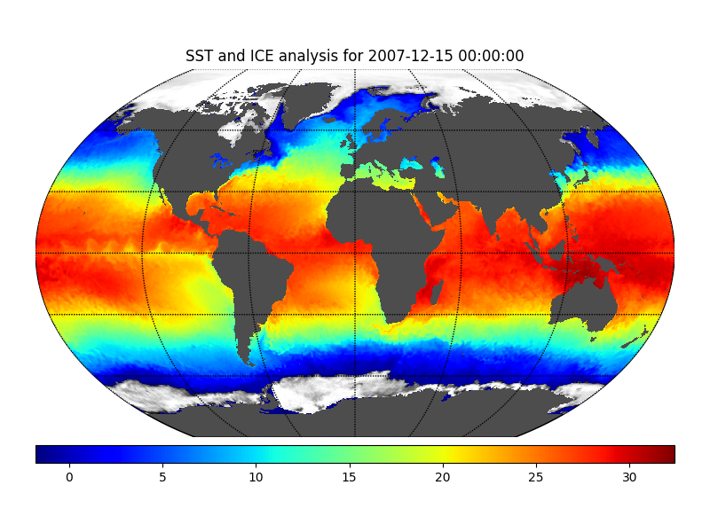
- Plotting wind vectors and wind barbs.
- 바람 벡터와 바람 barb를 플로팅.
import numpy as np
import matplotlib.pyplot as plt
import datetime
from mpl_toolkits.basemap import Basemap, shiftgrid
from netCDF4 import Dataset
# specify date to plot.
yyyy=1993; mm=3; dd=14; hh=0
date = datetime.datetime(yyyy,mm,dd,hh)
# set OpenDAP server URL.
URLbase="https://www.ncei.noaa.gov/thredds/dodsC/model-cfs_reanl_6h_pgb/"
URL=URLbase+"%04i/%04i%02i/%04i%02i%02i/pgbh00.gdas.%04i%02i%02i%02i.grb2" %\
             (yyyy,yyyy,mm,yyyy,mm,dd,yyyy,mm,dd,hh)
data = Dataset(URL)
# read lats,lons
# reverse latitudes so they go from south to north.
latitudes = data.variables['lat'][::-1]
longitudes = data.variables['lon'][:].tolist()
# get sea level pressure and 10-m wind data.
# mult slp by 0.01 to put in units of hPa.
slpin = 0.01*data.variables['Pressure_msl'][:].squeeze()
uin = data.variables['u-component_of_wind_height_above_ground'][:].squeeze()
vin = data.variables['v-component_of_wind_height_above_ground'][:].squeeze()
# add cyclic points manually (could use addcyclic function)
slp = np.zeros((slpin.shape[0],slpin.shape[1]+1),np.float64)
slp[:,0:-1] = slpin[::-1]; slp[:,-1] = slpin[::-1,0]
u = np.zeros((uin.shape[0],uin.shape[1]+1),np.float64)
u[:,0:-1] = uin[::-1]; u[:,-1] = uin[::-1,0]
v = np.zeros((vin.shape[0],vin.shape[1]+1),np.float64)
v[:,0:-1] = vin[::-1]; v[:,-1] = vin[::-1,0]
longitudes.append(360.); longitudes = np.array(longitudes)
# make 2-d grid of lons, lats
lons, lats = np.meshgrid(longitudes,latitudes)
# make orthographic basemap.
m = Basemap(resolution='c',projection='ortho',lat_0=60.,lon_0=-60.)
# create figure, add axes
fig1 = plt.figure(figsize=(8,10))
ax = fig1.add_axes([0.1,0.1,0.8,0.8])
# set desired contour levels.
clevs = np.arange(960,1061,5)
# compute native x,y coordinates of grid.
x, y = m(lons, lats)
# define parallels and meridians to draw.
parallels = np.arange(-80.,90,20.)
meridians = np.arange(0.,360.,20.)
# plot SLP contours.
CS1 = m.contour(x,y,slp,clevs,linewidths=0.5,colors='k')
CS2 = m.contourf(x,y,slp,clevs,cmap=plt.cm.RdBu_r)
# plot wind vectors on projection grid.
# first, shift grid so it goes from -180 to 180 (instead of 0 to 360
# in longitude).  Otherwise, interpolation is messed up.
ugrid,newlons = shiftgrid(180.,u,longitudes,start=False)
vgrid,newlons = shiftgrid(180.,v,longitudes,start=False)
# transform vectors to projection grid.
uproj,vproj,xx,yy = \
m.transform_vector(ugrid,vgrid,newlons,latitudes,31,31,returnxy=True,masked=True)
# now plot.
Q = m.quiver(xx,yy,uproj,vproj,scale=700)
# make quiver key.
qk = plt.quiverkey(Q, 0.1, 0.1, 20, '20 m/s', labelpos='W')
# draw coastlines, parallels, meridians.
m.drawcoastlines(linewidth=1.5)
m.drawparallels(parallels)
m.drawmeridians(meridians)
# add colorbar
cb = m.colorbar(CS2,"bottom", size="5%", pad="2%")
cb.set_label('hPa')
# set plot title
ax.set_title('SLP and Wind Vectors '+str(date))
plt.show()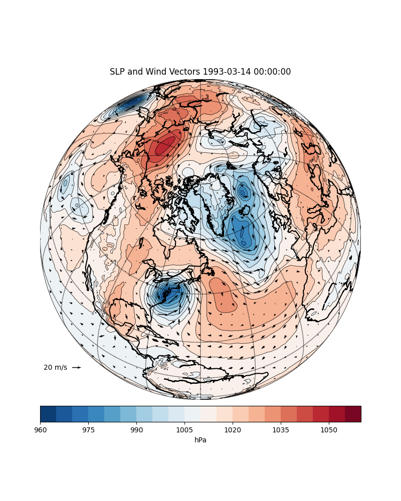
# create 2nd figure, add axes
fig2 = plt.figure(figsize=(8,10))
ax = fig2.add_axes([0.1,0.1,0.8,0.8])
# plot SLP contours
CS1 = m.contour(x,y,slp,clevs,linewidths=0.5,colors='k')
CS2 = m.contourf(x,y,slp,clevs,cmap=plt.cm.RdBu_r)
# plot wind barbs over map.
barbs = m.barbs(xx,yy,uproj,vproj,length=5,barbcolor='k',flagcolor='r',linewidth=0.5)
# draw coastlines, parallels, meridians.
m.drawcoastlines(linewidth=1.5)
m.drawparallels(parallels)
m.drawmeridians(meridians)
# add colorbar
cb = m.colorbar(CS2,"bottom", size="5%", pad="2%")
cb.set_label('hPa')
# set plot title.
ax.set_title('SLP and Wind Barbs '+str(date))
plt.show()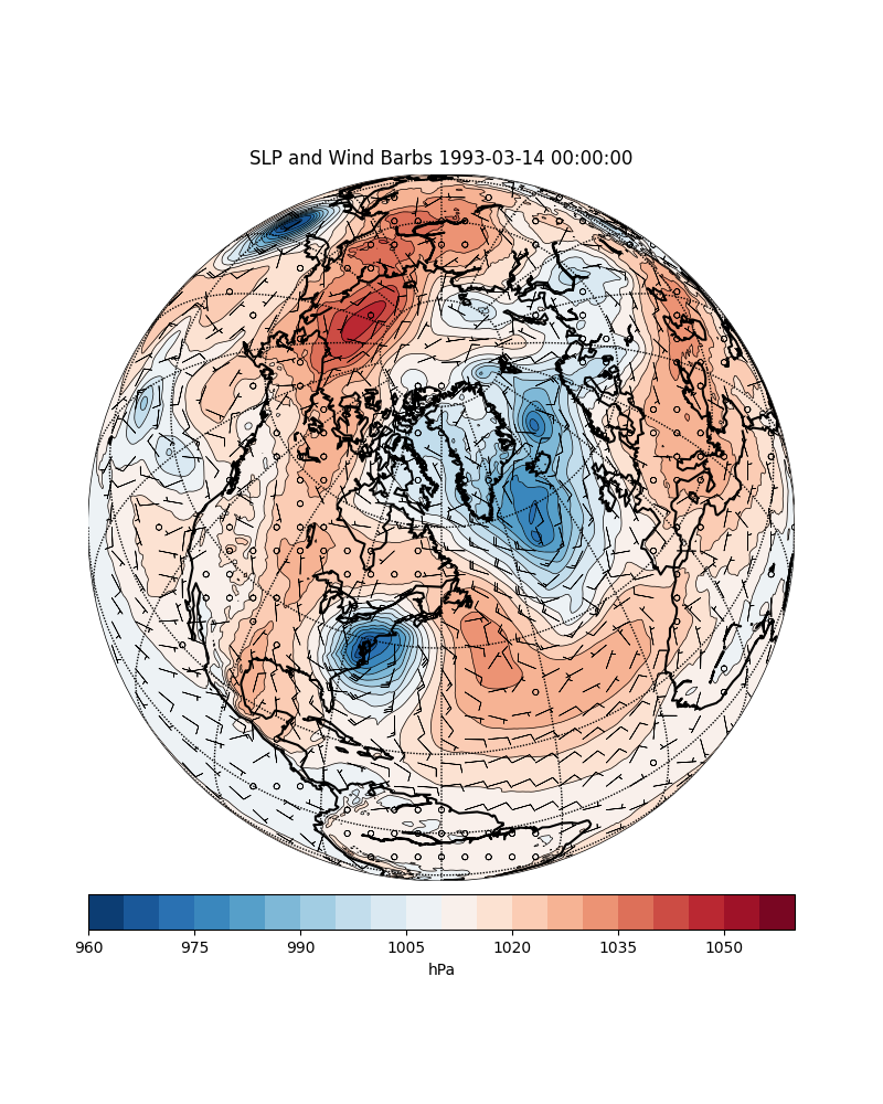
- Draw great circle between NY and London.
- 뉴욕과 런던 사이에 큰 원을 그린다.
from mpl_toolkits.basemap import Basemap
import numpy as np
import matplotlib.pyplot as plt
# create new figure, axes instances.
fig=plt.figure()
ax=fig.add_axes([0.1,0.1,0.8,0.8])
# setup mercator map projection.
m = Basemap(llcrnrlon=-100.,llcrnrlat=20.,urcrnrlon=20.,urcrnrlat=60.,\
            rsphere=(6378137.00,6356752.3142),\
            resolution='l',projection='merc',\
            lat_0=40.,lon_0=-20.,lat_ts=20.)
# nylat, nylon are lat/lon of New York
nylat = 40.78; nylon = -73.98
# lonlat, lonlon are lat/lon of London.
lonlat = 51.53; lonlon = 0.08
# draw great circle route between NY and London
m.drawgreatcircle(nylon,nylat,lonlon,lonlat,linewidth=2,color='b')
m.drawcoastlines()
m.fillcontinents()
# draw parallels
m.drawparallels(np.arange(10,90,20),labels=[1,1,0,1])
# draw meridians
m.drawmeridians(np.arange(-180,180,30),labels=[1,1,0,1])
ax.set_title('Great Circle from New York to London')
plt.show()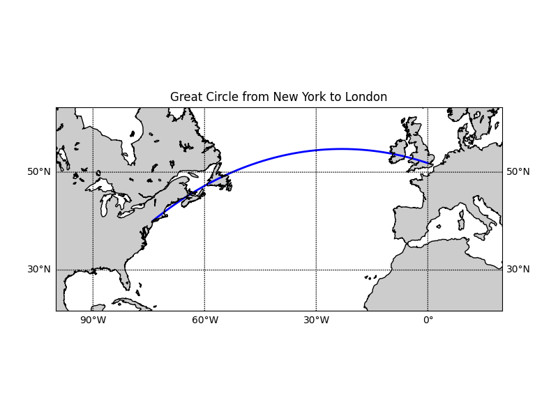
- Draw day-night terminator on a map.
- 지도에 낮과 밤의 terminator를 그린다.
import numpy as np from mpl_toolkits.basemap import Basemap import matplotlib.pyplot as plt from datetime import datetime # miller projection map = Basemap(projection='mill',lon_0=180) # plot coastlines, draw label meridians and parallels. map.drawcoastlines() map.drawparallels(np.arange(-90,90,30),labels=[1,0,0,0]) map.drawmeridians(np.arange(map.lonmin,map.lonmax+30,60),labels=[0,0,0,1]) # fill continents 'coral' (with zorder=0), color wet areas 'aqua' map.drawmapboundary(fill_color='aqua') map.fillcontinents(color='coral',lake_color='aqua') # shade the night areas, with alpha transparency so the # map shows through. Use current time in UTC. date = datetime.utcnow() CS=map.nightshade(date) plt.title('Day/Night Map for %s (UTC)' % date.strftime("%d %b %Y %H:%M:%S")) plt.show()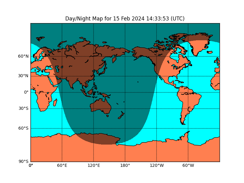 728x90
'코딩 > Python' 카테고리의 다른 글
Python/NumPy: the absolute basics for beginners (0) 2024.07.11 Python/NumPy/Quickstart (0) 2024.07.10 Python/지도를 사용할 수 있는 Folium/1. User guide (0) 2024.07.09 Python/지도를 사용할 수 있는 Folium/0. Getting started (0) 2024.07.09 Python/PyInstaller/0. PyInstaller Manual (0) 2024.07.08