Python/NumPy/Quickstart

https://numpy.org/doc/stable/user/quickstart.html의 번역본.

Prerequisites

You’ll need to know a bit of Python. For a refresher, see the Python tutorial.

To work the examples, you’ll need matplotlib installed in addition to NumPy.

Python을 조금 알아야 한다. 복습하려면 Python 튜토리얼을 참조하라.

예제를 작업하려면 NumPy 외에 matplotlib도 설치해야 한다.

Learner profile

This is a quick overview of arrays in NumPy. It demonstrates how n-dimensional ($n >= 2$) arrays are represented and can be manipulated. In particular, if you don’t know how to apply common functions to n-dimensional arrays (without using for-loops), or if you want to understand axis and shape properties for n-dimensional arrays, this article might be of help.

NumPy의 배열에 대한 간략한 개요이다. 이는 n차원(n >= 2) 배열이 표현되고 조작될 수 있다. 특히, for 루프를 사용하지 않고 n차원 배열에 일반 함수를 적용하는 방법을 모르거나 n차원 배열의 축 및 모양 속성을 이해하려는 경우 이 문서가 도움이 될 수 있다.

Learning Objectives

After reading, you should be able to:

• Understand the difference between one-, two- and n-dimensional arrays in NumPy;
• Understand how to apply some linear algebra operations to n-dimensional arrays without using for-loops;
• Understand axis and shape properties for n-dimensional arrays.

읽은 후에는 다음을 수행할 수 있어야 한다.

• NumPy의 1차원, 2차원 배열, n차원 배열의 차이점을 이해한다.
• for 루프를 사용하지 않고 n차원 배열에 일부 선형 대수 연산을 적용하는 방법을 이해한다.
• n차원 배열의 축 및 모양 속성을 이해한다.

The basics

NumPy’s main object is the homogeneous multidimensional array. It is a table of elements (usually numbers), all of the same type, indexed by a tuple of non-negative integers. In NumPy dimensions are called axes.

For example, the array for the coordinates of a point in 3D space, [1, 2, 1], has one axis. That axis has 3 elements in it, so we say it has a length of 3. In the example pictured below, the array has 2 axes. The first axis has a length of 2, the second axis has a length of 3.

NumPy의 주요 객체는 동종 다차원 배열이다. 이는 음이 아닌 정수의 튜플로 인덱싱된 동일한 유형의 요소(보통 숫자)의 테이블이다. NumPy에서는 차원을 축이라고 한다.

예를 들어 3D 공간의 한 점 좌표에 대한 배열 [1, 2, 1]에는 하나의 축이 있다. 해당 축에는 3개의 요소가 있으므로 길이가 3이라고 한다. 아래 그림의 예에서 배열에는 2개의 축이 있다. 첫 번째 축의 길이는 2이고, 두 번째 축의 길이는 3이다.

[[1., 0., 0.],
 [0., 1., 2.]]

NumPy’s array class is called ndarray. It is also known by the alias array. Note that numpy.array is not the same as the Standard Python Library class array.array, which only handles one-dimensional arrays and offers less functionality. The more important attributes of an ndarray object are:

NumPy의 배열 클래스는 ndarray라고 한다. 별칭 배열로도 알려져 있다. numpy.array는 1차원 배열만 처리하고 더 적은 기능을 제공하는 표준 Python 라이브러리 클래스 array.array와 동일하지 않다. ndarray 객체의 더 중요한 속성은 다음과 같다.

ndarray.ndim

the number of axes (dimensions) of the array.

배열의 축(차원) 수.

ndarray.shape

the dimensions of the array. This is a tuple of integers indicating the size of the array in each dimension. For a matrix with n rows and m columns, shape will be (n,m). The length of the shape tuple is therefore the number of axes, ndim.

배열의 차원. 이는 각 차원의 배열 크기를 나타내는 정수의 튜플이다. n행과 m열로 구성된 행렬의 경우 모양은 (n,m)이다. 따라서 모양 튜플의 길이는 축 수 ndim이다.

ndarray.size

the total number of elements of the array. This is equal to the product of the elements of shape.

배열의 총 요소 수. 이는 모양 요소의 곱과 같다.

ndarray.dtype

an object describing the type of the elements in the array. One can create or specify dtype’s using standard Python types. Additionally NumPy provides types of its own. numpy.int32, numpy.int16, and numpy.float64 are some examples.

배열의 요소 유형을 설명하는 객체. 표준 Python 유형을 사용하여 dtype을 생성하거나 지정할 수 있다. 또한 NumPy는 자체 유형을 제공한다. numpy.int32, numpy.int16 및 numpy.float64가 몇 가지 예이다.

ndarray.itemsize

the size in bytes of each element of the array. For example, an array of elements of type float64 has itemsize 8 (=64/8), while one of type complex32 has itemsize 4 (=32/8). It is equivalent to ndarray.dtype.itemsize.

배열의 각 요소의 크기(바이트). 예를 들어, float64 유형 요소 배열의 항목 크기는 8(=64/8)인 반면 complex32 유형 요소 배열의 항목 크기는 4(=32/8)이다. ndarray.dtype.itemsize와 동일하다.

ndarray.data

the buffer containing the actual elements of the array. Normally, we won’t need to use this attribute because we will access the elements in an array using indexing facilities.

배열의 실제 요소를 포함하는 버퍼. 일반적으로 우리는 인덱싱 기능을 사용하여 배열의 요소에 액세스하므로 이 속성을 사용할 필요가 없다.

An example

>>> import numpy as np
>>> a = np.arange(15).reshape(3, 5)
>>> a
array([[ 0,  1,  2,  3,  4],
       [ 5,  6,  7,  8,  9],
       [10, 11, 12, 13, 14]])
>>> a.shape
(3, 5)
>>> a.ndim
2
>>> a.dtype.name
'int64'
>>> a.itemsize
8
>>> a.size
15
>>> type(a)
<class 'numpy.ndarray'>
>>> b = np.array([6, 7, 8])
>>> b
array([6, 7, 8])
>>> type(b)
<class 'numpy.ndarray'>

Array creation

There are several ways to create arrays.

For example, you can create an array from a regular Python list or tuple using the array function. The type of the resulting array is deduced from the type of the elements in the sequences.

배열을 만드는 방법에는 여러 가지가 있다.

예를 들어, array 함수를 사용하여 일반 Python 목록이나 튜플에서 배열을 만들 수 있다. 결과 배열의 유형은 시퀀스의 요소 유형에서 추론된다.

>>> a = np.array([2, 3, 4])
>>> a
array([2, 3, 4])
>>> a.dtype
dtype('int64')
>>> b = np.array([1.2, 3.5, 5.1])
>>> b.dtype
dtype('float64')

A frequent error consists in calling array with multiple arguments, rather than providing a single sequence as an argument.

빈번한 오류는 단일 시퀀스를 인수로 제공하는 대신 여러 인수를 사용하여 배열을 호출하는 것이다.

>>> a = np.array(1, 2, 3, 4)    # WRONG
Traceback (most recent call last):
  ...
TypeError: array() takes from 1 to 2 positional arguments but 4 were given
a = np.array([1, 2, 3, 4])  # RIGHT

array transforms sequences of sequences into two-dimensional arrays, sequences of sequences of sequences into three-dimensional arrays, and so on.

배열은 시퀀스 시퀀스를 2차원 배열로 변환하고, 시퀀스 시퀀스의 시퀀스를 3차원 배열로 변환한다.

>>> b = np.array([(1.5, 2, 3), (4, 5, 6)])
>>> b
array([[1.5, 2. , 3. ],
       [4. , 5. , 6. ]])

The type of the array can also be explicitly specified at creation time:

배열 유형은 생성 시 명시적으로 지정할 수도 있다.

>>> c = np.array([[1, 2], [3, 4]], dtype=complex)
>>> c
array([[1.+0.j, 2.+0.j],
       [3.+0.j, 4.+0.j]])

Often, the elements of an array are originally unknown, but its size is known. Hence, NumPy offers several functions to create arrays with initial placeholder content. These minimize the necessity of growing arrays, an expensive operation.

The function zeros creates an array full of zeros, the function ones creates an array full of ones, and the function empty creates an array whose initial content is random and depends on the state of the memory. By default, the dtype of the created array is float64, but it can be specified via the key word argument dtype.

배열의 요소는 원래 알려지지 않았지만 크기는 알려진 경우가 많다. 따라서 NumPy는 초기 자리 표시자 내용으로 배열을 생성하는 여러 기능을 제공한다. 이는 비용이 많이 드는 작업인 Array 확장의 필요성을 최소화한다.

zeros 함수는 0으로 가득 찬 배열을 생성하고, ones 함수는 1로 가득 찬 배열을 생성하며, empty 함수는 초기 내용이 무작위이고 메모리 상태에 따라 달라지는 배열을 생성한다. 기본적으로 생성된 배열의 dtype은 float64이지만 키워드 인수 dtype을 통해 지정할 수 있다.

>>> np.zeros((3, 4))
array([[0., 0., 0., 0.],
       [0., 0., 0., 0.],
       [0., 0., 0., 0.]])
>>> np.ones((2, 3, 4), dtype=np.int16)
array([[[1, 1, 1, 1],
        [1, 1, 1, 1],
        [1, 1, 1, 1]],

       [[1, 1, 1, 1],
        [1, 1, 1, 1],
        [1, 1, 1, 1]]], dtype=int16)
>>> np.empty((2, 3))
array([[3.73603959e-262, 6.02658058e-154, 6.55490914e-260],  # may vary
       [5.30498948e-313, 3.14673309e-307, 1.00000000e+000]])

To create sequences of numbers, NumPy provides the arange function which is analogous to the Python built-in range, but returns an array.

일련의 숫자를 생성하기 위해 NumPy는 Python 내장 범위와 유사하지만 배열을 반환하는 arange 함수를 제공한다.

>>> np.arange(10, 30, 5)
array([10, 15, 20, 25])
>>> np.arange(0, 2, 0.3)  # it accepts float arguments
array([0. , 0.3, 0.6, 0.9, 1.2, 1.5, 1.8])

When arange is used with floating point arguments, it is generally not possible to predict the number of elements obtained, due to the finite floating point precision. For this reason, it is usually better to use the function linspace that receives as an argument the number of elements that we want, instead of the step:

부동 소수점 인수와 함께 arange를 사용하는 경우 유한한 부동 소수점 정밀도로 인해 일반적으로 획득된 요소 수를 예측하는 것이 불가능하다. 이러한 이유로 일반적으로 단계 대신 원하는 요소 수를 인수로 받는 linspace 함수를 사용하는 것이 더 좋다.

>>> from numpy import pi
>>> np.linspace(0, 2, 9)                   # 9 numbers from 0 to 2
array([0.  , 0.25, 0.5 , 0.75, 1.  , 1.25, 1.5 , 1.75, 2.  ])
>>> x = np.linspace(0, 2 * pi, 100)        # useful to evaluate function at lots of points
>>> f = np.sin(x)

See also

array, zeros, zeros_like, ones, ones_like, empty, empty_like, arange, linspace, random.Generator.random, random.Generator.normal, fromfunction, fromfile

Printing arrays

When you print an array, NumPy displays it in a similar way to nested lists, but with the following layout:

• the last axis is printed from left to right,
• the second-to-last is printed from top to bottom,
• the rest are also printed from top to bottom, with each slice separated from the next by an empty line.

배열을 인쇄할 때 NumPy는 이를 중첩 목록과 비슷한 방식으로 표시하지만 다음 레이아웃을 사용한다.

• 마지막 축은 왼쪽에서 오른쪽으로 인쇄된다.
• 마지막에서 두 번째는 위에서 아래로 인쇄된다.
• 나머지도 위에서 아래로 인쇄되며 각 조각은 빈 줄로 다음 조각과 구분된다.

One-dimensional arrays are then printed as rows, bidimensionals as matrices and tridimensionals as lists of matrices.

1차원 배열은 행으로, 2차원 배열은 행렬로, 3차원 배열은 행렬 목록으로 인쇄된다.

>>> a = np.arange(6)                    # 1d array
>>> print(a)
[0 1 2 3 4 5]

>>> b = np.arange(12).reshape(4, 3)     # 2d array
>>> print(b)
[[ 0  1  2]
 [ 3  4  5]
 [ 6  7  8]
 [ 9 10 11]]

>>> c = np.arange(24).reshape(2, 3, 4)  # 3d array
>>> print(c)
[[[ 0  1  2  3]
  [ 4  5  6  7]
  [ 8  9 10 11]]

 [[12 13 14 15]
  [16 17 18 19]
  [20 21 22 23]]]

See below to get more details on reshape.

If an array is too large to be printed, NumPy automatically skips the central part of the array and only prints the corners:

모양 변경에 대한 자세한 내용은 아래를 참조하라.

배열이 너무 커서 인쇄할 수 없으면 NumPy는 자동으로 배열의 중앙 부분을 건너뛰고 모서리만 인쇄한다.

>>> print(np.arange(10000))
[   0    1    2 ... 9997 9998 9999]

>>> print(np.arange(10000).reshape(100, 100))
[[   0    1    2 ...   97   98   99]
 [ 100  101  102 ...  197  198  199]
 [ 200  201  202 ...  297  298  299]
 ...
 [9700 9701 9702 ... 9797 9798 9799]
 [9800 9801 9802 ... 9897 9898 9899]
 [9900 9901 9902 ... 9997 9998 9999]]

To disable this behaviour and force NumPy to print the entire array, you can change the printing options using set_printoptions.

이 동작을 비활성화하고 NumPy가 전체 배열을 인쇄하도록 하려면 set_printoptions를 사용하여 인쇄 옵션을 변경할 수 있다.

import sys

np.set_printoptions(threshold=sys.maxsize)  # sys module should be imported

Basic operations

Arithmetic operators on arrays apply elementwise. A new array is created and filled with the result.

배열의 산술 연산자는 요소별로 적용된다. 새로운 배열이 생성되고 결과로 채워진다.

>>> a = np.array([20, 30, 40, 50])
>>> b = np.arange(4)
>>> b
array([0, 1, 2, 3])
>>> c = a - b
>>> c
array([20, 29, 38, 47])
>>> b**2
array([0, 1, 4, 9])
>>> 10 * np.sin(a)
array([ 9.12945251, -9.88031624,  7.4511316 , -2.62374854])
>>> a < 35
array([ True,  True, False, False])

Unlike in many matrix languages, the product operator * operates elementwise in NumPy arrays. The matrix product can be performed using the @ operator (in python >=3.5) or the dot function or method:

많은 행렬 언어와 달리 곱 연산자 *는 NumPy 배열에서 요소별로 작동한다. 행렬 곱은 @ 연산자(파이썬 >=3.5)나 도트 함수 또는 메서드를 사용하여 수행할 수 있다.

>>> A = np.array([[1, 1],
>>>               [0, 1]])
>>> B = np.array([[2, 0],
>>>               [3, 4]])
>>> A * B     # elementwise product
array([[2, 0],
       [0, 4]])
>>> A @ B     # matrix product
array([[5, 4],
       [3, 4]])
>>> A.dot(B)  # another matrix product
array([[5, 4],
       [3, 4]])

Some operations, such as += and *=, act in place to modify an existing array rather than create a new one.

+= 및 *=와 같은 일부 작업은 새 배열을 생성하는 대신 기존 배열을 수정하는 역할을 한다.

>>> rg = np.random.default_rng(1)  # create instance of default random number generator
>>> a = np.ones((2, 3), dtype=int)
>>> b = rg.random((2, 3))
>>> a *= 3
>>> a
array([[3, 3, 3],
       [3, 3, 3]])
>>> b += a
>>> b
array([[3.51182162, 3.9504637 , 3.14415961],
       [3.94864945, 3.31183145, 3.42332645]])
>>> a += b  # b is not automatically converted to integer type
Traceback (most recent call last):
    ...
numpy._core._exceptions._UFuncOutputCastingError: Cannot cast ufunc 'add' output from dtype
('float64') to dtype('int64') with casting rule 'same_kind'

When operating with arrays of different types, the type of the resulting array corresponds to the more general or precise one (a behavior known as upcasting).

다양한 유형의 배열로 작업할 때 결과 배열의 유형은 보다 일반적이거나 정확한 유형에 해당한다(업캐스팅이라는 동작).

>>> a = np.ones(3, dtype=np.int32)
>>> b = np.linspace(0, pi, 3)
>>> b.dtype.name
'float64'
>>> c = a + b
>>> c
array([1.        , 2.57079633, 4.14159265])
>>> c.dtype.name
'float64'
>>> d = np.exp(c * 1j)
>>> d
array([ 0.54030231+0.84147098j, -0.84147098+0.54030231j,
       -0.54030231-0.84147098j])
>>> d.dtype.name
'complex128'

Many unary operations, such as computing the sum of all the elements in the array, are implemented as methods of the ndarray class.

배열에 있는 모든 요소의 합을 계산하는 것과 같은 많은 단항 연산은 ndarray 클래스의 메서드로 구현된다.

>>> a = rg.random((2, 3))
>>> a
array([[0.82770259, 0.40919914, 0.54959369],
       [0.02755911, 0.75351311, 0.53814331]])
>>> a.sum()
3.1057109529998157
>>> a.min()
0.027559113243068367
>>> a.max()
0.8277025938204418

By default, these operations apply to the array as though it were a list of numbers, regardless of its shape. However, by specifying the axis parameter you can apply an operation along the specified axis of an array:

기본적으로 이러한 작업은 모양에 관계없이 숫자 목록인 것처럼 배열에 적용된다. 그러나 axis 매개변수를 지정하면 배열의 지정된 축을 따라 작업을 적용할 수 있다.

>>> b = np.arange(12).reshape(3, 4)
>>> b
array([[ 0,  1,  2,  3],
       [ 4,  5,  6,  7],
       [ 8,  9, 10, 11]])

>>> b.sum(axis=0)     # sum of each column
array([12, 15, 18, 21])

>>> b.min(axis=1)     # min of each row
array([0, 4, 8])

>>> b.cumsum(axis=1)  # cumulative sum along each row
array([[ 0,  1,  3,  6],
       [ 4,  9, 15, 22],
       [ 8, 17, 27, 38]])

Universal functions

NumPy provides familiar mathematical functions such as sin, cos, and exp. In NumPy, these are called “universal functions” (ufunc). Within NumPy, these functions operate elementwise on an array, producing an array as output.

NumPy는 sin, cos, exp와 같은 친숙한 수학 함수를 제공한다. NumPy에서는 이를 "유니버설 함수"(ufunc)라고 한다. NumPy 내에서 이러한 함수는 배열에서 요소별로 작동하여 배열을 출력으로 생성한다.

>>> B = np.arange(3)
>>> B
array([0, 1, 2])
>>> np.exp(B)
array([1.        , 2.71828183, 7.3890561 ])
>>> np.sqrt(B)
array([0.        , 1.        , 1.41421356])
>>> C = np.array([2., -1., 4.])
>>> np.add(B, C)
array([2., 0., 6.])

See also

all, any, apply_along_axis, argmax, argmin, argsort, average, bincount, ceil, clip, conj, corrcoef, cov, cross, cumprod, cumsum, diff, dot, floor, inner, invert, lexsort, max, maximum, mean, median, min, minimum, nonzero, outer, prod, re, round, sort, std, sum, trace, transpose, var, vdot, vectorize, where

Indexing, slicing and iterating

One-dimensional arrays can be indexed, sliced and iterated over, much like lists and other Python sequences.

1차원 배열은 목록 및 기타 Python 시퀀스와 마찬가지로 인덱싱, 슬라이싱 및 반복이 가능하다.

>>> a = np.arange(10)**3
>>> a
array([  0,   1,   8,  27,  64, 125, 216, 343, 512, 729])
>>> a[2]
8
>>> a[2:5]
array([ 8, 27, 64])
>>> # equivalent to a[0:6:2] = 1000;
>>> # from start to position 6, exclusive, set every 2nd element to 1000
>>> a[:6:2] = 1000
>>> a
array([1000,    1, 1000,   27, 1000,  125,  216,  343,  512,  729])
>>> a[::-1]  # reversed a
array([ 729,  512,  343,  216,  125, 1000,   27, 1000,    1, 1000])
>>> for i in a:
>>>     print(i**(1 / 3.))

9.999999999999998  # may vary
1.0
9.999999999999998
3.0
9.999999999999998
4.999999999999999
5.999999999999999
6.999999999999999
7.999999999999999
8.999999999999998

Multidimensional arrays can have one index per axis. These indices are given in a tuple separated by commas:

다차원 배열은 축당 하나의 인덱스를 가질 수 있다. 이러한 인덱스는 쉼표로 구분된 튜플로 제공된다.

>>> def f(x, y):
>>>     return 10 * x + y

>>> b = np.fromfunction(f, (5, 4), dtype=int)
>>> b
array([[ 0,  1,  2,  3],
       [10, 11, 12, 13],
       [20, 21, 22, 23],
       [30, 31, 32, 33],
       [40, 41, 42, 43]])
>>> b[2, 3]
23
>>> b[0:5, 1]  # each row in the second column of b
array([ 1, 11, 21, 31, 41])
>>> b[:, 1]    # equivalent to the previous example
array([ 1, 11, 21, 31, 41])
>>> b[1:3, :]  # each column in the second and third row of b
array([[10, 11, 12, 13],
       [20, 21, 22, 23]])

When fewer indices are provided than the number of axes, the missing indices are considered complete slices:

축 수보다 적은 수의 인덱스가 제공되면 누락된 인덱스는 완전한 조각으로 간주된다.

>>> b[-1]   # the last row. Equivalent to b[-1, :]
array([40, 41, 42, 43])

The expression within brackets in b[i] is treated as an i followed by as many instances of : as needed to represent the remaining axes. NumPy also allows you to write this using dots as b[i, ...].

The dots (...) represent as many colons as needed to produce a complete indexing tuple. For example, if x is an array with 5 axes, then

• x[1, 2, ...] is equivalent to x[1, 2, :, :, :],
• x[..., 3] to x[:, :, :, :, 3] and
• x[4, ..., 5, :] to x[4, :, :, 5, :].

b[i]의 대괄호 안의 표현식은 i와 나머지 축을 나타내는 데 필요한 만큼의 : 인스턴스로 처리된다. NumPy를 사용하면 점을 사용하여 b[i, ...]로 작성할 수도 있다.

점(...)은 완전한 인덱싱 튜플을 생성하는 데 필요한 만큼의 콜론을 나타낸다. 예를 들어, x가 5개의 축을 가진 배열이면

• x[1, 2, ...]는 x[1, 2, :, :, :]와 동일하다.
• x[..., 3]에서 x[:, :, :, :, 3] 및
• x[4, ..., 5, :]에서 x[4, :, :, 5, :].

>>> c = np.array([[[  0,  1,  2],  # a 3D array (two stacked 2D arrays)
>>>                [ 10, 12, 13]],
>>>               [[100, 101, 102],
>>>                [110, 112, 113]]])
>>> c.shape
(2, 2, 3)
>>> c[1, ...]  # same as c[1, :, :] or c[1]
array([[100, 101, 102],
       [110, 112, 113]])
>>> c[..., 2]  # same as c[:, :, 2]
array([[  2,  13],
       [102, 113]])

Iterating over multidimensional arrays is done with respect to the first axis:

다차원 배열에 대한 반복은 첫 번째 축을 기준으로 수행된다.

>>> for row in b:
>>>     print(row)

[0 1 2 3]
[10 11 12 13]
[20 21 22 23]
[30 31 32 33]
[40 41 42 43]

However, if one wants to perform an operation on each element in the array, one can use the flat attribute which is an iterator over all the elements of the array:

그러나 배열의 각 요소에 대해 작업을 수행하려는 경우 배열의 모든 요소에 대한 반복자인 flat 속성을 사용할 수 있다.

>>> for element in b.flat:
>>>     print(element)

0
1
2
3
10
11
12
13
20
21
22
23
30
31
32
33
40
41
42
43

See also

Indexing on ndarrays, Indexing routines (reference), newaxis, ndenumerate, indices

Shape manipulation

Changing the shape of an array

An array has a shape given by the number of elements along each axis:

배열은 각 축의 요소 수에 따라 모양이 지정된다.

>>> a = np.floor(10 * rg.random((3, 4)))
>>> a
array([[3., 7., 3., 4.],
       [1., 4., 2., 2.],
       [7., 2., 4., 9.]])
>>> a.shape
(3, 4)

The shape of an array can be changed with various commands. Note that the following three commands all return a modified array, but do not change the original array:

다양한 명령을 사용하여 배열의 모양을 변경할 수 있다. 다음 세 가지 명령은 모두 수정된 배열을 반환하지만 원래 배열은 변경하지 않는다.

>>> a.ravel()  # returns the array, flattened
array([3., 7., 3., 4., 1., 4., 2., 2., 7., 2., 4., 9.])
>>> a.reshape(6, 2)  # returns the array with a modified shape
array([[3., 7.],
       [3., 4.],
       [1., 4.],
       [2., 2.],
       [7., 2.],
       [4., 9.]])
>>> a.T  # returns the array, transposed
array([[3., 1., 7.],
       [7., 4., 2.],
       [3., 2., 4.],
       [4., 2., 9.]])
>>> a.T.shape
(4, 3)
>>> a.shape
(3, 4)

The order of the elements in the array resulting from ravel is normally “C-style”, that is, the rightmost index “changes the fastest”, so the element after a[0, 0] is a[0, 1]. If the array is reshaped to some other shape, again the array is treated as “C-style”. NumPy normally creates arrays stored in this order, so ravel will usually not need to copy its argument, but if the array was made by taking slices of another array or created with unusual options, it may need to be copied. The functions ravel and reshape can also be instructed, using an optional argument, to use FORTRAN-style arrays, in which the leftmost index changes the fastest.

The reshape function returns its argument with a modified shape, whereas the ndarray.resize method modifies the array itself:

ravel로 인해 발생하는 배열 요소의 순서는 일반적으로 "C 스타일"이다. 즉, 가장 오른쪽 인덱스가 "가장 빠르게 변경"되므로 a[0, 0] 뒤의 요소는 a[0, 1]이다. 배열이 다른 모양으로 변경되면 배열은 다시 "C 스타일"로 처리된다. NumPy는 일반적으로 이 순서로 저장된 배열을 생성하므로 ravel은 일반적으로 인수를 복사할 필요가 없지만, 배열이 다른 배열의 슬라이스를 사용하여 생성되었거나 특이한 옵션으로 생성된 경우 복사해야 할 수 있다. 선택적 인수를 사용하여 ravel 및 reshape 함수에 가장 왼쪽 인덱스가 가장 빠르게 변경되는 FORTRAN 스타일 배열을 사용하도록 지시할 수도 있다.

reshape 함수는 수정된 모양으로 인수를 반환하는 반면, ndarray.resize 메서드는 배열 자체를 수정한다.

>>> a
array([[3., 7., 3., 4.],
       [1., 4., 2., 2.],
       [7., 2., 4., 9.]])
>>> a.resize((2, 6))
>>> a
array([[3., 7., 3., 4., 1., 4.],
       [2., 2., 7., 2., 4., 9.]])

If a dimension is given as -1 in a reshaping operation, the other dimensions are automatically calculated:

재형성 작업에서 차원이 -1로 지정되면 다른 차원이 자동으로 계산된다.

>>> a.reshape(3, -1)
array([[3., 7., 3., 4.],
       [1., 4., 2., 2.],
       [7., 2., 4., 9.]])

See also

ndarray.shape, reshape, resize, ravel

Stacking together different arrays

Several arrays can be stacked together along different axes:

여러 배열을 서로 다른 축을 따라 함께 쌓을 수 있다.

>>> a = np.floor(10 * rg.random((2, 2)))
>>> a
array([[9., 7.],
       [5., 2.]])
>>> b = np.floor(10 * rg.random((2, 2)))
>>> b
array([[1., 9.],
       [5., 1.]])
>>> np.vstack((a, b))
array([[9., 7.],
       [5., 2.],
       [1., 9.],
       [5., 1.]])
>>> np.hstack((a, b))
array([[9., 7., 1., 9.],
       [5., 2., 5., 1.]])

The function column_stack stacks 1D arrays as columns into a 2D array. It is equivalent to hstack only for 2D arrays:

column_stack 함수는 1D 배열을 2D 배열의 열로 쌓는다. 2D 배열의 경우에만 hstack과 동일하다.

>>> from numpy import newaxis
>>> np.column_stack((a, b))  # with 2D arrays
array([[9., 7., 1., 9.],
       [5., 2., 5., 1.]])
>>> a = np.array([4., 2.])
>>> b = np.array([3., 8.])
>>> np.column_stack((a, b))  # returns a 2D array
array([[4., 3.],
       [2., 8.]])
>>> np.hstack((a, b))        # the result is different
array([4., 2., 3., 8.])
>>> a[:, newaxis]  # view `a` as a 2D column vector
array([[4.],
       [2.]])
>>> np.column_stack((a[:, newaxis], b[:, newaxis]))
array([[4., 3.],
       [2., 8.]])
>>> np.hstack((a[:, newaxis], b[:, newaxis]))  # the result is the same
array([[4., 3.],
       [2., 8.]])

In general, for arrays with more than two dimensions, hstack stacks along their second axes, vstack stacks along their first axes, and concatenate allows for an optional arguments giving the number of the axis along which the concatenation should happen.

일반적으로 2차원 이상의 배열의 경우 hstack은 두 번째 축을 따라 스택되고, vstack은 첫 번째 축을 따라 스택되며, concatenate는 연결이 발생해야 하는 축 수를 제공하는 선택적 인수를 허용한다.

Note

In complex cases, r_ and c_ are useful for creating arrays by stacking numbers along one axis. They allow the use of range literals :.

복잡한 경우 r_ 및 c_는 한 축을 따라 숫자를 쌓아 배열을 만드는 데 유용하다. 범위 리터럴을 사용할 수 있다.

np.r_[1:4, 0, 4]
array([1, 2, 3, 0, 4])

When used with arrays as arguments, r_ and c_ are similar to vstack and hstack in their default behavior, but allow for an optional argument giving the number of the axis along which to concatenate.

배열을 인수로 사용하는 경우 r_ 및 c_는 기본 동작에서 vstack 및 hstack과 유사하지만 연결할 축 수를 제공하는 선택적 인수를 허용한다.

See also

hstack, vstack, column_stack, concatenate, c_, r_

Splitting one array into several smaller ones

Using hsplit, you can split an array along its horizontal axis, either by specifying the number of equally shaped arrays to return, or by specifying the columns after which the division should occur:

hsplit을 사용하면 반환할 동일한 모양의 배열 수를 지정하거나 분할이 발생해야 하는 열을 지정하여 가로 축을 따라 배열을 분할할 수 있다.

>>> a = np.floor(10 * rg.random((2, 12)))
>>> a
array([[6., 7., 6., 9., 0., 5., 4., 0., 6., 8., 5., 2.],
       [8., 5., 5., 7., 1., 8., 6., 7., 1., 8., 1., 0.]])
>>> # Split `a` into 3
>>> np.hsplit(a, 3)
[array([[6., 7., 6., 9.],
       [8., 5., 5., 7.]]), array([[0., 5., 4., 0.],
       [1., 8., 6., 7.]]), array([[6., 8., 5., 2.],
       [1., 8., 1., 0.]])]
>>> # Split `a` after the third and the fourth column
>>> np.hsplit(a, (3, 4))
[array([[6., 7., 6.],
       [8., 5., 5.]]), array([[9.],
       [7.]]), array([[0., 5., 4., 0., 6., 8., 5., 2.],
       [1., 8., 6., 7., 1., 8., 1., 0.]])]

vsplit splits along the vertical axis, and array_split allows one to specify along which axis to split.

vsplit은 수직 축을 따라 분할되며 array_split을 사용하면 분할할 축을 지정할 수 있다.

Copies and views

When operating and manipulating arrays, their data is sometimes copied into a new array and sometimes not. This is often a source of confusion for beginners. There are three cases:

Array를 작동하고 조작할 때 해당 데이터가 새 Array에 복사되는 경우도 있고 복사되지 않는 경우도 있다. 이는 종종 초보자에게 혼란의 원인이 된다. 세 가지 경우가 있다:

No copy at all

Simple assignments make no copy of objects or their data.

단순 할당은 개체나 해당 데이터의 복사본을 만들지 않는다.

>>> a = np.array([[ 0,  1,  2,  3],
>>>               [ 4,  5,  6,  7],
>>>               [ 8,  9, 10, 11]])
>>> b = a            # no new object is created
>>> b is a           # a and b are two names for the same ndarray object
True

Python passes mutable objects as references, so function calls make no copy.

Python은 변경 가능한 객체를 참조로 전달하므로 함수 호출은 복사본을 만들지 않는다.

>>> def f(x):
>>>     print(id(x))

>>> id(a)  # id is a unique identifier of an object
148293216  # may vary
>>> f(a)
148293216  # may vary

View or shallow copy

Different array objects can share the same data. The view method creates a new array object that looks at the same data.

서로 다른 배열 객체가 동일한 데이터를 공유할 수 있다. view 메소드는 동일한 데이터를 보는 새로운 배열 객체를 생성한다.

>>> c = a.view()
>>> c is a
False
>>> c.base is a            # c is a view of the data owned by a
True
>>> c.flags.owndata
False

>>> c = c.reshape((2, 6))  # a's shape doesn't change
>>> a.shape
(3, 4)
>>> c[0, 4] = 1234         # a's data changes
>>> a
array([[   0,    1,    2,    3],
       [1234,    5,    6,    7],
       [   8,    9,   10,   11]])

Slicing an array returns a view of it:

배열을 슬라이싱하면 해당 배열의 뷰가 반환된다.

>>> s = a[:, 1:3]
>>> s[:] = 10  # s[:] is a view of s. Note the difference between s = 10 and s[:] = 10
>>> a
array([[   0,   10,   10,    3],
       [1234,   10,   10,    7],
       [   8,   10,   10,   11]])

Deep copy

The copy method makes a complete copy of the array and its data.

copy 메소드는 배열과 해당 데이터의 전체 복사본을 만든다.

>>> d = a.copy()  # a new array object with new data is created
>>> d is a
False
>>> d.base is a  # d doesn't share anything with a
False
>>> d[0, 0] = 9999
>>> a
array([[   0,   10,   10,    3],
       [1234,   10,   10,    7],
       [   8,   10,   10,   11]])

Sometimes copy should be called after slicing if the original array is not required anymore. For example, suppose a is a huge intermediate result and the final result b only contains a small fraction of a, a deep copy should be made when constructing b with slicing:

원본 배열이 더 이상 필요하지 않은 경우 슬라이싱 후에 복사본을 호출해야 하는 경우도 있다. 예를 들어, a가 거대한 중간 결과이고 최종 결과 b에 ​​a의 작은 부분만 포함되어 있다고 가정하면 슬라이싱을 사용하여 b를 구성할 때 깊은 복사본을 만들어야 한다.

>>> a = np.arange(int(1e8))
>>> b = a[:100].copy()
>>> del a  # the memory of ``a`` can be released.

If b = a[:100] is used instead, a is referenced by b and will persist in memory even if del a is executed.

대신 b = a[:100]을 사용하면 a는 b에서 참조되며 del a가 실행되더라도 메모리에 유지된다.

Functions and methods overview

Here is a list of some useful NumPy functions and methods names ordered in categories. See Routines and objects by topic for the full list.

다음은 카테고리별로 정렬된 몇 가지 유용한 NumPy 함수 및 메소드 이름 목록이다. 전체 목록은 주제별 루틴 및 개체를 참조하라.

Array Creation

arange, array, copy, empty, empty_like, eye, fromfile, fromfunction, identity, linspace, logspace, mgrid, ogrid, ones, ones_like, r_, zeros, zeros_like

Conversions

ndarray.astype, atleast_1d, atleast_2d, atleast_3d, mat

Manipulations

array_split, column_stack, concatenate, diagonal, dsplit, dstack, hsplit, hstack, ndarray.item, newaxis, ravel, repeat, reshape, resize, squeeze, swapaxes, take, transpose, vsplit, vstack

Questions

all, any, nonzero, where

Ordering

argmax, argmin, argsort, max, min, ptp, searchsorted, sort

Operations

choose, compress, cumprod, cumsum, inner, ndarray.fill, imag, prod, put, putmask, real, sum

Basic Statistics

cov, mean, std, var

Basic Linear Algebra

cross, dot, outer, linalg.svd, vdot

Less basic

Broadcasting rules

Broadcasting allows universal functions to deal in a meaningful way with inputs that do not have exactly the same shape.

The first rule of broadcasting is that if all input arrays do not have the same number of dimensions, a “1” will be repeatedly prepended to the shapes of the smaller arrays until all the arrays have the same number of dimensions.

The second rule of broadcasting ensures that arrays with a size of 1 along a particular dimension act as if they had the size of the array with the largest shape along that dimension. The value of the array element is assumed to be the same along that dimension for the “broadcast” array.

After application of the broadcasting rules, the sizes of all arrays must match. More details can be found in Broadcasting.

브로드캐스팅을 사용하면 범용 함수가 정확히 동일한 모양을 갖지 않는 입력을 의미 있는 방식으로 처리할 수 있다.

브로드캐스팅의 첫 번째 규칙은 모든 입력 배열의 차원 수가 동일하지 않은 경우 모든 배열이 동일한 차원 수를 가질 때까지 더 작은 배열의 모양 앞에 "1"이 반복적으로 추가된다는 것이다.

브로드캐스트의 두 번째 규칙은 특정 차원을 따라 크기가 1인 배열이 해당 차원을 따라 가장 큰 모양의 배열 크기를 갖는 것처럼 작동하도록 보장한다. 배열 요소의 값은 "브로드캐스트" 배열의 해당 차원에서 동일한 것으로 간주된다.

브로드캐스트 규칙을 적용한 후에는 모든 배열의 크기가 일치해야 한다. 자세한 내용은 방송에서 확인할 수 있다.

Advanced indexing and index tricks

NumPy offers more indexing facilities than regular Python sequences. In addition to indexing by integers and slices, as we saw before, arrays can be indexed by arrays of integers and arrays of booleans.

NumPy는 일반 Python 시퀀스보다 더 많은 인덱싱 기능을 제공한다. 앞에서 본 것처럼 정수와 슬라이스로 인덱싱하는 것 외에도 배열은 정수 배열과 부울 배열로 인덱싱할 수 있다.

Indexing with arrays of indices

>>> a = np.arange(12)**2  # the first 12 square numbers
>>> i = np.array([1, 1, 3, 8, 5])  # an array of indices
>>> a[i]  # the elements of `a` at the positions `i`
array([ 1,  1,  9, 64, 25])

>>> j = np.array([[3, 4], [9, 7]])  # a bidimensional array of indices
>>> a[j]  # the same shape as `j`
array([[ 9, 16],
       [81, 49]])

When the indexed array a is multidimensional, a single array of indices refers to the first dimension of a. The following example shows this behavior by converting an image of labels into a color image using a palette.

인덱스 배열 a가 다차원인 경우 단일 인덱스 배열은 a의 첫 번째 차원을 참조한다. 다음 예에서는 팔레트를 사용하여 레이블 이미지를 컬러 이미지로 변환하여 이 동작을 보여준다.

>>> palette = np.array([[0, 0, 0],         # black
>>>                     [255, 0, 0],       # red
>>>                     [0, 255, 0],       # green
>>>                     [0, 0, 255],       # blue
>>>                     [255, 255, 255]])  # white
>>> image = np.array([[0, 1, 2, 0],  # each value corresponds to a color in the palette
>>>                   [0, 3, 4, 0]])
>>> palette[image]  # the (2, 4, 3) color image
array([[[  0,   0,   0],
        [255,   0,   0],
        [  0, 255,   0],
        [  0,   0,   0]],

       [[  0,   0,   0],
        [  0,   0, 255],
        [255, 255, 255],
        [  0,   0,   0]]])

We can also give indexes for more than one dimension. The arrays of indices for each dimension must have the same shape.

또한 둘 이상의 차원에 대한 인덱스를 제공할 수도 있다. 각 차원의 인덱스 배열은 동일한 모양을 가져야 한다.

>>> a = np.arange(12).reshape(3, 4)
>>> a
array([[ 0,  1,  2,  3],
       [ 4,  5,  6,  7],
       [ 8,  9, 10, 11]])
>>> i = np.array([[0, 1],  # indices for the first dim of `a`
>>>               [1, 2]])
>>> j = np.array([[2, 1],  # indices for the second dim
>>>               [3, 3]])

>>> a[i, j]  # i and j must have equal shape
array([[ 2,  5],
       [ 7, 11]])

>>> a[i, 2]
array([[ 2,  6],
       [ 6, 10]])

>>> a[:, j]
array([[[ 2,  1],
        [ 3,  3]],

       [[ 6,  5],
        [ 7,  7]],

       [[10,  9],
        [11, 11]]])

In Python, arr[i, j] is exactly the same as arr[(i, j)]—so we can put i and j in a tuple and then do the indexing with that.

Python에서 arr[i, j]는 arr[(i, j)]와 정확히 동일하므로 i와 j를 튜플에 넣은 다음 이를 사용하여 인덱싱을 수행할 수 있다.

>>> l = (i, j)
>>> # equivalent to a[i, j]
>>> a[l]
array([[ 2,  5],
       [ 7, 11]])

However, we can not do this by putting i and j into an array, because this array will be interpreted as indexing the first dimension of a.

그러나 i와 j를 배열에 넣어서 이를 수행할 수는 없다. 왜냐하면 이 배열은 a의 첫 번째 차원을 인덱싱하는 것으로 해석되기 때문이다.

>>> s = np.array([i, j])
>>> # not what we want
>>> a[s]
Traceback (most recent call last):
  File "", line 1, in 
IndexError: index 3 is out of bounds for axis 0 with size 3
>>> # same as `a[i, j]`
>>> a[tuple(s)]
array([[ 2,  5],
       [ 7, 11]])

Another common use of indexing with arrays is the search of the maximum value of time-dependent series:

배열을 사용한 인덱싱의 또 다른 일반적인 용도는 시간 종속 계열의 최대값을 검색하는 것이다.

>>> time = np.linspace(20, 145, 5)  # time scale
>>> data = np.sin(np.arange(20)).reshape(5, 4)  # 4 time-dependent series
>>> time
array([ 20.  ,  51.25,  82.5 , 113.75, 145.  ])
>>> data
array([[ 0.        ,  0.84147098,  0.90929743,  0.14112001],
       [-0.7568025 , -0.95892427, -0.2794155 ,  0.6569866 ],
       [ 0.98935825,  0.41211849, -0.54402111, -0.99999021],
       [-0.53657292,  0.42016704,  0.99060736,  0.65028784],
       [-0.28790332, -0.96139749, -0.75098725,  0.14987721]])
>>> # index of the maxima for each series
>>> ind = data.argmax(axis=0)
>>> ind
array([2, 0, 3, 1])
>>> # times corresponding to the maxima
>>> time_max = time[ind]

>>> data_max = data[ind, range(data.shape[1])]  # => data[ind[0], 0], data[ind[1], 1]...
>>> time_max
array([ 82.5 ,  20.  , 113.75,  51.25])
>>> data_max
array([0.98935825, 0.84147098, 0.99060736, 0.6569866 ])
>>> np.all(data_max == data.max(axis=0))
True

You can also use indexing with arrays as a target to assign to:

배열을 사용하여 인덱싱을 대상으로 할당할 수도 있다.

>>> a = np.arange(5)
>>> a
array([0, 1, 2, 3, 4])
>>> a[[1, 3, 4]] = 0
>>> a
array([0, 0, 2, 0, 0])

However, when the list of indices contains repetitions, the assignment is done several times, leaving behind the last value:

그러나 인덱스 목록에 반복이 포함된 경우 할당이 여러 번 수행되어 마지막 값이 남는다.

>>> a = np.arange(5)
>>> a[[0, 0, 2]] = [1, 2, 3]
>>> a
array([2, 1, 3, 3, 4])

This is reasonable enough, but watch out if you want to use Python’s += construct, as it may not do what you expect:

이는 충분히 합리적이지만 Python의 += 구문을 사용하려는 경우 예상한 대로 작동하지 않을 수 있으므로 주의하라.

>>> a = np.arange(5)
>>> a[[0, 0, 2]] += 1
>>> a
array([1, 1, 3, 3, 4])

Even though 0 occurs twice in the list of indices, the 0th element is only incremented once. This is because Python requires a += 1 to be equivalent to a = a + 1.

인덱스 목록에 0이 두 번 발생하더라도 0번째 요소는 한 번만 증가한다. 이는 Python에서 a = a + 1과 동일하려면 += 1이 필요하기 때문이다.

Indexing with boolean arrays

When we index arrays with arrays of (integer) indices we are providing the list of indices to pick. With boolean indices the approach is different; we explicitly choose which items in the array we want and which ones we don’t.

The most natural way one can think of for boolean indexing is to use boolean arrays that have the same shape as the original array:

(정수) 인덱스 배열로 배열을 인덱싱할 때 선택할 인덱스 목록을 제공한다. 부울 인덱스를 사용하면 접근 방식이 다르다. 배열에서 원하는 항목과 원하지 않는 항목을 명시적으로 선택한다.

부울 인덱싱에 대해 생각할 수 있는 가장 자연스러운 방법은 원래 배열과 모양이 동일한 부울 배열을 사용하는 것이다.

>>> a = np.arange(12).reshape(3, 4)
>>> b = a > 4
>>> b  # `b` is a boolean with `a`'s shape
array([[False, False, False, False],
       [False,  True,  True,  True],
       [ True,  True,  True,  True]])
>>> a[b]  # 1d array with the selected elements
array([ 5,  6,  7,  8,  9, 10, 11])

This property can be very useful in assignments:

이 속성은 할당에 매우 유용할 수 있다.

>>> a[b] = 0  # All elements of `a` higher than 4 become 0
>>> a
array([[0, 1, 2, 3],
       [4, 0, 0, 0],
       [0, 0, 0, 0]])

You can look at the following example to see how to use boolean indexing to generate an image of the Mandelbrot set:

다음 예를 보면 부울 인덱싱을 사용하여 만델브로 집합의 이미지를 생성하는 방법을 확인할 수 있다.

def mandelbrot(h, w, maxit=20, r=2):
    """Returns an image of the Mandelbrot fractal of size (h,w)."""
    x = np.linspace(-2.5, 1.5, 4*h+1)
    y = np.linspace(-1.5, 1.5, 3*w+1)
    A, B = np.meshgrid(x, y)
    C = A + B*1j
    z = np.zeros_like(C)
    divtime = maxit + np.zeros(z.shape, dtype=int)

    for i in range(maxit):
       z = z**2 + C
       diverge = abs(z) > r                    # who is diverging
       div_now = diverge & (divtime == maxit)  # who is diverging now
       divtime[div_now] = i                    # note when
       z[diverge] = r                          # avoid diverging too much

    return divtime
plt.clf()
plt.imshow(mandelbrot(400, 400))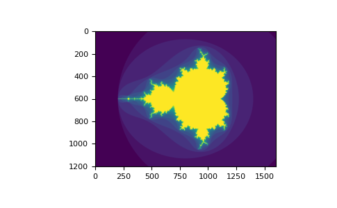

The second way of indexing with booleans is more similar to integer indexing; for each dimension of the array we give a 1D boolean array selecting the slices we want:

부울을 사용하여 인덱싱하는 두 번째 방법은 정수 인덱싱과 더 유사하다. 배열의 각 차원에 대해 원하는 슬라이스를 선택하는 1D 부울 배열을 제공한다.

>>> a = np.arange(12).reshape(3, 4)
>>> b1 = np.array([False, True, True])         # first dim selection
>>> b2 = np.array([True, False, True, False])  # second dim selection

>>> a[b1, :]                                   # selecting rows
array([[ 4,  5,  6,  7],
       [ 8,  9, 10, 11]])

>>> a[b1]                                      # same thing
array([[ 4,  5,  6,  7],
       [ 8,  9, 10, 11]])

>>> a[:, b2]                                   # selecting columns
array([[ 0,  2],
       [ 4,  6],
       [ 8, 10]])

>>> a[b1, b2]                                  # a weird thing to do
array([ 4, 10])

Note that the length of the 1D boolean array must coincide with the length of the dimension (or axis) you want to slice. In the previous example, b1 has length 3 (the number of rows in a), and b2 (of length 4) is suitable to index the 2nd axis (columns) of a.

1D 부울 배열의 길이는 슬라이스하려는 차원(또는 축)의 길이와 일치해야 한다. 이전 예에서 b1의 길이는 3(a의 행 수)이고 b2(길이 4)는 a의 두 번째 축(열)을 인덱싱하는 데 적합하다.

The ix_() function

The ix_ function can be used to combine different vectors so as to obtain the result for each n-uplet. For example, if you want to compute all the a+b*c for all the triplets taken from each of the vectors a, b and c:

ix_ 함수는 서로 다른 벡터를 결합하여 각 n-uplet에 대한 결과를 얻는 데 사용할 수 있다. 예를 들어, 각 벡터 a, b 및 c에서 가져온 모든 삼중항에 대해 모든 a+b*c를 계산하려는 경우:

>>> a = np.array([2, 3, 4, 5])
>>> b = np.array([8, 5, 4])
>>> c = np.array([5, 4, 6, 8, 3])
>>> ax, bx, cx = np.ix_(a, b, c)
>>> ax
array([[[2]],

       [[3]],

       [[4]],

       [[5]]])
>>> bx
array([[[8],
        [5],
        [4]]])
>>> cx
array([[[5, 4, 6, 8, 3]]])
>>> ax.shape, bx.shape, cx.shape
((4, 1, 1), (1, 3, 1), (1, 1, 5))
>>> result = ax + bx * cx
>>> result
array([[[42, 34, 50, 66, 26],
        [27, 22, 32, 42, 17],
        [22, 18, 26, 34, 14]],

       [[43, 35, 51, 67, 27],
        [28, 23, 33, 43, 18],
        [23, 19, 27, 35, 15]],

       [[44, 36, 52, 68, 28],
        [29, 24, 34, 44, 19],
        [24, 20, 28, 36, 16]],

       [[45, 37, 53, 69, 29],
        [30, 25, 35, 45, 20],
        [25, 21, 29, 37, 17]]])
>>> result[3, 2, 4]
17
>>> a[3] + b[2] * c[4]
17

You could also implement the reduce as follows:

다음과 같이 축소를 구현할 수도 있다.

def ufunc_reduce(ufct, *vectors):
   vs = np.ix_(*vectors)
   r = ufct.identity
   for v in vs:
       r = ufct(r, v)
   return r

and then use it as:

그런 다음 다음과 같이 사용하라.

>>> ufunc_reduce(np.add, a, b, c)
array([[[15, 14, 16, 18, 13],
        [12, 11, 13, 15, 10],
        [11, 10, 12, 14,  9]],

       [[16, 15, 17, 19, 14],
        [13, 12, 14, 16, 11],
        [12, 11, 13, 15, 10]],

       [[17, 16, 18, 20, 15],
        [14, 13, 15, 17, 12],
        [13, 12, 14, 16, 11]],

       [[18, 17, 19, 21, 16],
        [15, 14, 16, 18, 13],
        [14, 13, 15, 17, 12]]])

The advantage of this version of reduce compared to the normal ufunc.reduce is that it makes use of the broadcasting rules in order to avoid creating an argument array the size of the output times the number of vectors.

일반 ufunc.reduce와 비교하여 이 버전의 축소의 장점은 출력 크기와 벡터 수를 곱한 인수 배열 생성을 피하기 위해 브로드캐스팅 규칙을 사용한다는 것이다.

Indexing with strings

See Structured arrays.

구조적 배열을 참조하라.

Tricks and tips

Here we give a list of short and useful tips.

여기서는 짧고 유용한 팁 목록을 제공한다.

“Automatic” reshaping

To change the dimensions of an array, you can omit one of the sizes which will then be deduced automatically:

배열의 크기를 변경하려면 자동으로 추론되는 크기 중 하나를 생략하면 된다.

>>> a = np.arange(30)
>>> b = a.reshape((2, -1, 3))  # -1 means "whatever is needed"
>>> b.shape
(2, 5, 3)
>>> b
array([[[ 0,  1,  2],
        [ 3,  4,  5],
        [ 6,  7,  8],
        [ 9, 10, 11],
        [12, 13, 14]],

       [[15, 16, 17],
        [18, 19, 20],
        [21, 22, 23],
        [24, 25, 26],
        [27, 28, 29]]])

Vector stacking

How do we construct a 2D array from a list of equally-sized row vectors? In MATLAB this is quite easy: if x and y are two vectors of the same length you only need do m=[x;y]. In NumPy this works via the functions column_stack, dstack, hstack and vstack, depending on the dimension in which the stacking is to be done. For example:

동일한 크기의 행 벡터 목록에서 2D 배열을 어떻게 구성하는가? MATLAB에서는 이는 매우 쉽다. x와 y가 동일한 길이의 두 벡터인 경우 m=[x;y]만 수행하면 된다. NumPy에서는 스태킹이 수행되는 차원에 따라 column_stack, dstack, hstack 및 vstack 함수를 통해 작동한다. 예를 들어:

>>> x = np.arange(0, 10, 2)
>>> y = np.arange(5)
>>> m = np.vstack([x, y])
>>> m
array([[0, 2, 4, 6, 8],
       [0, 1, 2, 3, 4]])
>>> xy = np.hstack([x, y])
>>> xy
array([0, 2, 4, 6, 8, 0, 1, 2, 3, 4])

The logic behind those functions in more than two dimensions can be strange.

2차원 이상의 기능에 대한 논리는 이상할 수 있다.

See also

NumPy for MATLAB users

Histograms

The NumPy histogram function applied to an array returns a pair of vectors: the histogram of the array and a vector of the bin edges. Beware: matplotlib also has a function to build histograms (called hist, as in Matlab) that differs from the one in NumPy. The main difference is that pylab.hist plots the histogram automatically, while numpy.histogram only generates the data.

배열에 적용된 NumPy 히스토그램 함수는 한 쌍의 벡터, 즉 배열의 히스토그램과 빈 가장자리의 벡터를 반환한다. 주의: matplotlib에는 NumPy의 기능과 다른 히스토그램(Matlab에서는 hist라고 함)을 작성하는 기능도 있다. 주요 차이점은 pylab.hist가 자동으로 히스토그램을 그리는 반면 numpy.histogram은 데이터만 생성한다는 것이다.

rg = np.random.default_rng(1)
import matplotlib.pyplot as plt
# Build a vector of 10000 normal deviates with variance 0.5^2 and mean 2
mu, sigma = 2, 0.5
v = rg.normal(mu, sigma, 10000)
# Plot a normalized histogram with 50 bins
plt.hist(v, bins=50, density=True)       # matplotlib version (plot)
# Compute the histogram with numpy and then plot it
(n, bins) = np.histogram(v, bins=50, density=True)  # NumPy version (no plot)
plt.plot(.5 * (bins[1:] + bins[:-1]), n)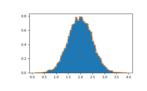

With Matplotlib >=3.4 you can also use plt.stairs(n, bins).

Matplotlib >=3.4를 사용하면 plt.stairs(n, bins)를 사용할 수도 있다.